How to Create a Checklist in Microsoft Excel
 Sandy Writtenhouse

Sandy Writtenhouse
Writer
With her B.S. in Information Technology, Sandy worked for many years in the IT industry as a Project Manager, Department Manager, and PMO Lead. She learned how technology can enrich both professional and personal lives by using the right tools. And, she has shared those suggestions and how-tos on many websites over time. With thousands of articles under her belt, Sandy strives to help others use technology to their advantage. Read more.

If you’re building a spreadsheet to share with others or simply one for your own tracking, using a checklist can make data entry a breeze in Microsoft Excel. Here’s how to create a checklist in your spreadsheet and make it look like your own.
Why a checklist? You might use a checklist for tracking items to pack for a trip, products for your company, a holiday gift list, monthly bills, or keeping track of tasks. With a simple check box form control, you can create a checklist for anything you like in Excel.
Access the Developer Tab
Before you can use the check box form control in Microsoft Excel, you need to make sure that you have access to the Developer tab. If you don’t see this tab at the top of Excel, it takes only a minute to add it.
Right-click anywhere on your Excel ribbon and select “Customize the Ribbon” from the drop-down list. Alternatively, you can click File > Options > Customize Ribbon from the menu.

On the right side of the window, under “Customize the Ribbon,” make sure “Main Tabs” is selected. Then in the list below it, check the box next to the “Developer” option.

Click “OK” and then close the Excel Options window.
Add Your List of Items in Excel
The best way to begin your checklist is to add the list items. Even though you can always add or remove items later, this gives you the start you need to add your checkboxes. And you can, of course, add any row or column headers that you need.

Add Check Boxes for Your List Items
The action part of a checklist is the checkbox. And this is where the Developer tab comes into the mix, so be sure to select that tab. Go to an item on your list and click the cell next to it where you want a checkbox.
In the “”Controls” section of the ribbon, click the “Insert” button. Pick the “Checkbox” option in the “Form Controls” area.

You’ll then see your cursor change to crosshairs (like a plus sign). Drag a corner, and when you see your checkbox display, release.

By default, the checkbox will have a label attached to it which you will not need for a basic checklist. Select that text and hit your “Backspace” or “Delete” key. You can then select the checkbox control and drag a corner to resize it if needed.

Format Your Checkboxes
Once you insert a checkbox, you can make changes to its appearance if you like. Right-click the checkbox control. Make sure that you right-click the actual control and not the cell containing it. Select “Format Control” in the shortcut menu.

You’ll see tabs for “Colors and Lines” and “Size,” which give you easy ways to color the lines, add a fill color, scale the checkbox, and lock the aspect ratio. Be sure to click “OK” after making your changes.

Checkbox Values and Cell Links
The other tab you may want to work with is the “Control” tab. This one lets you set the value, add a cell link if necessary, and apply 3D shading.
Checkbox Values
By default, a checkbox is unchecked when you insert it. Depending on the type of checklist you create, you might want the boxes checked by default instead. This forces the user to uncheck items they don’t want. To do this, mark “Checked” under “Value” in the Control tab and click “OK.”

Cell Links
If you plan to use your checklist in conjunction with Microsoft Excel formulas, you’ll likely use “Cell Link” on the “Control” tab. When you enter a cell into this box, it will display a True or False value based on the box being checked or unchecked.
Here’s an example. Say your checklist has 25 items and you plan to use the COUNTIF function to see how many of the items are checked. You can base your formula off of the True and False values associated with the checked and unchecked boxes.
To use the “Cell Link,” simply type the cell reference into the box or click the cell in your spreadsheet to populate it automatically.

Add the Remaining Checkboxes
Follow the above steps to add checkboxes to your remaining list items. Or for a quicker way, use AutoFill to copy the checkboxes through the cells of your other items.
To use AutoFill, put your cursor on the bottom-right corner of the cell containing the checkbox. When you see the Fill Handle (plus sign), drag to fill the additional cells and release.

For marking off a list of to-dos, making a gift list and checking it twice, or tracking bills you pay each month, creating a checklist in Excel is a great way to go!
And if you like the list idea, how about adding a drop-down list in Microsoft Excel too?
- › How to Create a Basic Form in Microsoft Excel
- › How to Create a Custom List in Microsoft Excel
- › How to Insert a Check Mark in Microsoft Excel
- › How to Use Microsoft Excel Templates for Event Planning
- › How to Add a Checkbox in Google Sheets
- › How to Count Checkboxes in Microsoft Excel
- › How to Insert a Checkbox in Microsoft Excel
- › Mac Gaming Is About To Get Much Better. Here’s Why
 Sandy Writtenhouse
With her B.S. in Information Technology, Sandy worked for many years in the IT industry as a Project Manager, Department Manager, and PMO Lead. She learned how technology can enrich both professional and personal lives by using the right tools. And, she has shared those suggestions and how-tos on many websites over time. With thousands of articles under her belt, Sandy strives to help others use technology to their advantage.
Read Full Bio »
Как создать удобный чек-лист (контрольный список) в Excel, чтобы ничего не забыть
Excel – довольно удобный инструмент с обширным функционалом. Множество приложений предлагают возможность создавать различные списки, но зачем пользоваться другими программами, если есть Excel?

Как создать удобный чек-лист (контрольный список) в Excel
Ниже мы покажем, как создать таблицу с флажками, которые вы можете удалять по мере выполнения задач. Excel даже отобразит, когда вы снимете все флажки. Создать таблицу довольно просто. Для этого нужно открыть вкладку «Разработчик», внести список задач, добавить флажки и расширенное форматирование. А теперь по порядку.
1. Открыть вкладку «Разработчик»
По умолчанию вкладка «Разработчик» не отображается. Ее можно добавить в ленту следующим образом: откройте «Файл» → «Параметры» → «Настроить ленту». В списке «Основные вкладки» установите флажок «Разработчик», а затем нажмите «Готово».

2. Добавление списка задач в таблицу
В каждой ячейке таблицы укажите задачу. В нашем примере одна из ячеек будет содержать «Общее количество предметов», вторая – «Упакованные предметы». Ячейка «Я готов» будет отображаться красным, если не все галочки в списке сняты, и зеленым, если флажки сняты все.
Откройте вкладку «Разработчик». Нажмите «Вставить» и в разделе «Элементы управления формы» выберите «Флажок» (иконку с галочкой).

3. Добавление флажков
Кликните на ячейку, в которую хотите добавить флажок. Вы увидите, что справа от поля флажка отображается текст. Так как нам нужно только поле, выделите текст и удалите его. После удаления текста размер поля не изменяется автоматически.

Если вы хотите изменить его, щелкните правой кнопкой мыши по ячейке, чтобы выбрать поле, а затем левой кнопкой мыши щелкните по нему. Таким образом вы сможете изменить его размеры и переместить на середину ячейки. Для того чтобы скопировать поле флажка и разместить его в других ячейках, выберите ячейку, а затем используйте кнопки управления курсором (клавиши со стрелками на клавиатуре) для перемещения к ячейке с флажком. Для того чтобы скопировать поле флажка в другие ячейки, наведите курсор в нижний угол ячейки, захватите его кнопкой мыши и протяните по ячейкам, в которые нужно скопировать поле. Отпустите кнопку мыши.

Расширенное форматирование списка
В зависимости от предназначения списка вы можете использовать расширенное форматирование.
Создание столбца ИСТИНА/ЛОЖЬ
Для этого нужно использовать колонку справа от полей с флажками. Флажок будет возвращать ИСТИНА (если галочка установлена) или ЛОЖЬ (если она снята). Таким образом вы сможете увидеть, все ли флажки сняты.
Правой кнопкой мыши нажмите на первое поле флажка и выберите «Формат объекта».

На вкладке «Элемент управления» в окне «Формат объекта» нажмите на кнопку выбора ячейки с правой стороны поля «Связь с ячейкой».

Выберите ячейку, которая находится справа от клетки с флажком. Адрес выбранной ячейки размещен в поле «Связь с ячейкой» в компактной версии окна «Формат объекта», чтобы развернуть его повторно нажмите на кнопку «Связь с ячейкой» и выберите «ОК». Повторите указанную процедуру для каждой ячейки в списке.

Общее число предметов и подсчет отмеченных предметов в списке
Укажите общее количество флажков в списке в ячейке, расположенной справа от клетки «Общее количество предметов». Число проставленных галочек можно подсчитать с помощью специальной функции. Введите
=СЧЁТЕСЛИ(C2:C8; ИСТИНА)
=COUNTIF(C2:C8,TRUE)
в ячейку справа от ячейки «Упакованные предметы» и нажмите Enter. Как показано в примере ниже, функция подсчитает число ячеек в колонке С (с С2 по С8), имеющих значение ИСТИНА или TRUE.

Скрыть столбец ИСТИНА/ЛОЖЬ
Для того чтобы скрыть данную колонку, правой кнопкой мыши кликните на ее заголовке и в отобразившемся меню выберите пункт «Скрыть». Столбец будет скрыт.

Как проверить, все ли галочки сняты
Для этого выберите ячейку «Я готов» и введите
=ЕСЛИ(B10=B11;»Да»;»Нет»)
=IF(B10=B11,»YES»,»NO»)
Если число в ячейке В10 совпадет со значением подсчитанных флажков в ячейке В11, в ней автоматически отобразится «Да», в противном случае появится «Нет».

Применение условного форматирования
С помощью условного форматирования вы можете выделить ячейки цветом. К примеру, вы можете задать условное форматирование таким образом, чтобы все ячейки со значениями определенного типа закрашивались в красный цвет.
Создайте правило, открыв «Главная» → «Условное форматирование» → «Создать правило» → «Диспетчер правил условного форматирования» → «Использовать формулу для определения форматируемых ячеек». Введите
в поле «Форматировать значения, для которых следующая формула является истинной:». Замените значения В10 и В11 адресами ячеек «Общее количество предметов» и «Упакованные предметы», если это не одни и те же ячейки.

Создайте еще одно правило, но в поле «Форматировать значения, для которых следующая формула является истинной:» введите формулу
=$B10=$B11
Затем нажмите «Формат», выберите цвет и нажмите «ОК».
В окне «Диспетчер правил условного форматирования» введите адреса ячеек, которые должны быть заполнены цветом, в поле «Применяется к». Введите те же адреса для обоих правил. В нашем случае это =$B$13. Нажмите «ОК».

Ячейка «Я готов» окрасится зеленым цветом, если все галочки будут сняты, или красным, если нет.
How To Make A Checklist In Excel In 5 Easy Steps
Whether it’s a grocery list or your daily task list at work, a checklist ensures that you get everything done.
And while there are a number of native and online checklist apps as well as templates that you can use to manage your work, you can easily create one using everyday tools like Microsoft Excel. And that’s what you’ll learn today:
How to create a checklist in Excel
Unlike Microsoft Word, Excel has had form controls right from the 2007 version. So the steps below work for both—Excel 2007 and 2010.
1. Enable the Developer menu
In Excel, you can insert a checkbox control from the Developer menu. However, this menu isn’t enabled by default.

You can enable the Developer menu in Excel 2010 with the following steps:
- Open the Excel Options dialog box by navigating to File → Options.
- Click on the Customize Ribbon option.
- Check the Developer checkbox in the Main Tabs control.

- Open the Excel Options dialog box by clicking on the Microsoft Office button → Excel Options.
- Click on the Popular option.
- Check the Show Developer tab in the Ribbon checkbox.
2. Add your checklist items
Next, begin your checklist by adding items to it.

You can easily add new items, update an item, or remove items from the checklist. Plus, you can reorder the items by dragging and dropping the rows in the Excel spreadsheet.
3. Insert checkboxes next to the items
The checkbox next to a list item is what makes your checklist actionable.

To add a checkbox:
- Navigate to the Developer tab in the spreadsheet’s Ribbon menu.
- Next, click on the Insert dropdown menu.
- Finally, click on the checkbox to insert it into a cell next to a list item.
Alternatively, you can also use the radio button control.
The checkbox control comes with its own label attached. This is useful for simple checklists. Alternatively, you can also delete the label text and display just a checkbox control.
Finally, copy and paste the checkbox control across all the list items. As an alternative, you can also use the Excel Fill Handle to drag and fill the checkbox across all list items.
4. Make your checkbox look good
This step is optional. But sometimes you may want your checkbox to have a different size or color.

To change the checkbox appearance:
- Right-click on the checkbox and open the Format Control dialog box.
- On the dialog box you can change the following properties of the checkbox control:
- Colors and line styles
- Size (height and width)
- The default state—checked, unchecked, or mixed
- And more
5. Run through your checklist
Finally, it’s time to run through your checklist.

You can either print the checklist and use your pen or alternatively click on the checkbox to mark the items done.
Excel checklist templates
If you want to use a readymade checklist template for Excel, you have a number of options available on the internet.
Here are two of my favorite ones:
Cheery Checklist Template
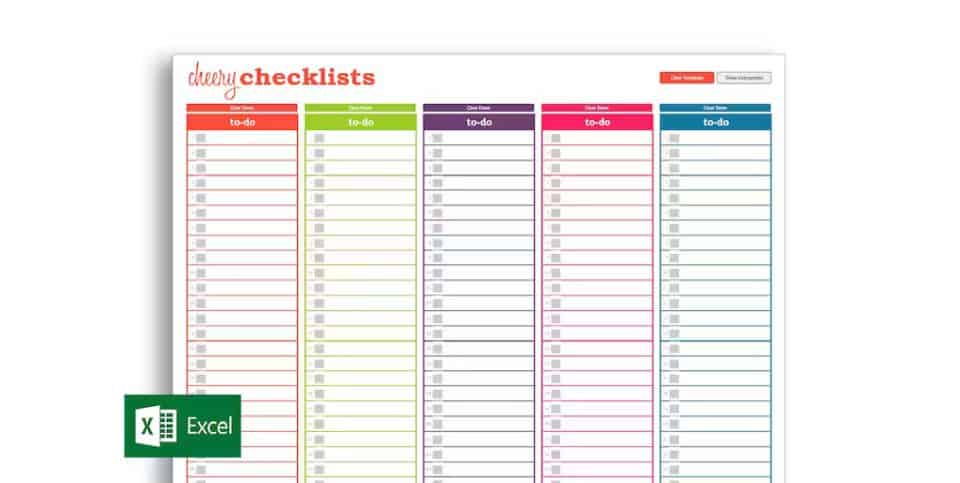
This flexible, colorful Excel checklist template is available on Etsy for $11.80.
It comes with five colorful checklists, one for a project. You can edit the titles of these checklists. And, each checklist has 24 to-do items.
It works with Excel 2010 or newer on PC and the 2016+ versions on Mac.
Free Daily Checklist
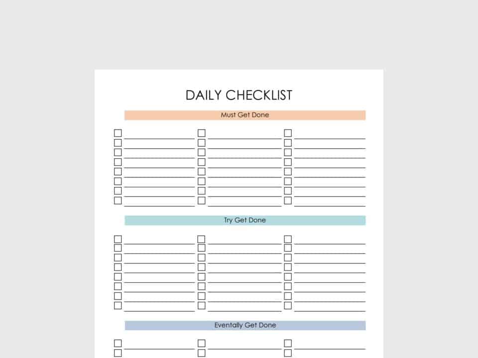
This Daily Checklist template for Excel is available for free along with 30 other templates.
It comes with three sections to prioritize your to-do items—Must get done, Try to get done, and eventually get done.
Each section can hold up to 24 to-do items.
Pros and cons of Excel checklists
Excel checklists are great if you want something quick and cheap. Plus, everyone has access and knows how to use it.
However, there are some serious drawbacks as well:
- Collaboration is hard. Sharing a copy of the file with your team and then recompiling it every time can quickly get tiring.
- Anyone can mark a list item done. So keeping track of who’s updating what can become impossible.
- No way to add more details to a to-do item. You cannot attach files or provide feedback.
How do you get around this, particularly for teams?
By using one of the many checklist apps available today. These online apps make it easy to plan, track, and manage all your work tasks along with your team.
Toggl Plan is one such app. It’s a beautifully simple work management tool that makes planning and tracking tasks easy.

Add task details and attach a checklist to tasks in Toggl Plan
You can add task details, attach files, and add feedback comments right on the task. Plus you can attach a checklist to a task to ensure that each task gets done according to the expected quality.
Best of all you can plan tasks on a timeline and quickly detect scheduling conflicts if any.
Jitesh is an SEO and content specialist. He manages content projects at Toggl and loves sharing actionable tips to deliver projects profitably.
Как сделать чек лист в Excel?
Сперва перейдите на вкладку Разработчик (Developer), чтобы иметь возможность создать чеклист. Нажмите кнопку Вставить (Insert). Затем из раздела Элементы управления формы (Form Controls section) выберите Флажок (Check Box).Oct 4, 2015
Что такое чек лист и как его составить?
Чек лист — это список пунктов, составленный в произвольном порядке. Он может обозначать последовательность шагов для выполнения задачи, список важных дел, характеристики объекта. Чек лист может быть составлен на бумаге, электронном носителе, маркерной доске. Вы хотя бы раз в жизни составляли чек-лист.