Linear algebra ( numpy.linalg )#
The NumPy linear algebra functions rely on BLAS and LAPACK to provide efficient low level implementations of standard linear algebra algorithms. Those libraries may be provided by NumPy itself using C versions of a subset of their reference implementations but, when possible, highly optimized libraries that take advantage of specialized processor functionality are preferred. Examples of such libraries are OpenBLAS, MKL (TM), and ATLAS. Because those libraries are multithreaded and processor dependent, environmental variables and external packages such as threadpoolctl may be needed to control the number of threads or specify the processor architecture.
The SciPy library also contains a linalg submodule, and there is overlap in the functionality provided by the SciPy and NumPy submodules. SciPy contains functions not found in numpy.linalg , such as functions related to LU decomposition and the Schur decomposition, multiple ways of calculating the pseudoinverse, and matrix transcendentals such as the matrix logarithm. Some functions that exist in both have augmented functionality in scipy.linalg . For example, scipy.linalg.eig can take a second matrix argument for solving generalized eigenvalue problems. Some functions in NumPy, however, have more flexible broadcasting options. For example, numpy.linalg.solve can handle “stacked” arrays, while scipy.linalg.solve accepts only a single square array as its first argument.
The term matrix as it is used on this page indicates a 2d numpy.array object, and not a numpy.matrix object. The latter is no longer recommended, even for linear algebra. See the matrix object documentation for more information.
The @ operator#
Introduced in NumPy 1.10.0, the @ operator is preferable to other methods when computing the matrix product between 2d arrays. The numpy.matmul function implements the @ operator.
Matrix and vector products#
Dot product of two arrays.
Compute the dot product of two or more arrays in a single function call, while automatically selecting the fastest evaluation order.
Return the dot product of two vectors.
Inner product of two arrays.
Compute the outer product of two vectors.
matmul (x1, x2, /[, out, casting, order, . ])
Matrix product of two arrays.
Compute tensor dot product along specified axes.
einsum (subscripts, *operands[, out, dtype, . ])
Evaluates the Einstein summation convention on the operands.
einsum_path (subscripts, *operands[, optimize])
Evaluates the lowest cost contraction order for an einsum expression by considering the creation of intermediate arrays.
Raise a square matrix to the (integer) power n.
Kronecker product of two arrays.
Decompositions#
Compute the qr factorization of a matrix.
linalg.svd (a[, full_matrices, compute_uv, . ])
Singular Value Decomposition.
Matrix eigenvalues#
Compute the eigenvalues and right eigenvectors of a square array.
Return the eigenvalues and eigenvectors of a complex Hermitian (conjugate symmetric) or a real symmetric matrix.
Compute the eigenvalues of a general matrix.
Compute the eigenvalues of a complex Hermitian or real symmetric matrix.
Norms and other numbers#
Matrix or vector norm.
Compute the condition number of a matrix.
Compute the determinant of an array.
Return matrix rank of array using SVD method
Compute the sign and (natural) logarithm of the determinant of an array.
trace (a[, offset, axis1, axis2, dtype, out])
Return the sum along diagonals of the array.
Solving equations and inverting matrices#
Solve a linear matrix equation, or system of linear scalar equations.
Solve the tensor equation a x = b for x.
Return the least-squares solution to a linear matrix equation.
Compute the (multiplicative) inverse of a matrix.
Compute the (Moore-Penrose) pseudo-inverse of a matrix.
Compute the ‘inverse’ of an N-dimensional array.
Exceptions#
Generic Python-exception-derived object raised by linalg functions.
Linear algebra on several matrices at once#
New in version 1.8.0.
Several of the linear algebra routines listed above are able to compute results for several matrices at once, if they are stacked into the same array.
Introduction
In this chapter, we will see what is the meaning of the determinant of a matrix. This special number can tell us a lot of things about our matrix!
2.11 The determinant
We saw in 2.8 that a matrix can be seen as a linear transformation of the space. The determinant of a matrix $\bs$ is a number corresponding to the multiplicative change you get when you transform your space with this matrix (see a comment by Pete L. Clark in this SE question). A negative determinant means that there is a change in orientation (and not just a rescaling and/or a rotation). As outlined by Nykamp DQ on Math Insight, a change in orientation means for instance in 2D that we take a plane out of these 2 dimensions, do some transformations and get back to the initial 2D space. Here is an example distinguishing between positive and negative determinant:
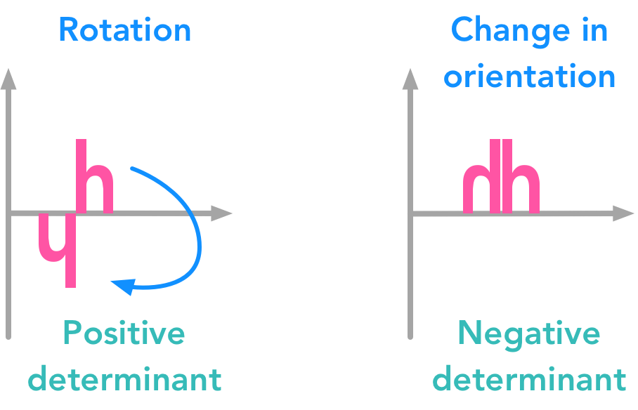
The determinant of a matrix can tell you a lot of things about the transformation associated with this matrix
You can see that the second transformation can’t be obtained through rotation and rescaling. Thus the sign can tell you the nature of the transformation associated with the matrix!
Example 1.
To calculate the area of the shapes, we will use simple squares in 2 dimensions. The unit square area can be calculated with the Pythagorean theorem taking the two unit vectors.
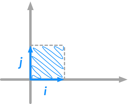
The unit square area
The lengths of $i$ and $j$ are $1$ thus the area of the unit square is $1$.
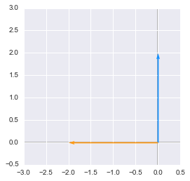
First, let’s create a function plotVectors() to plot vectors:
And let’s start by creating both vectors in Python:
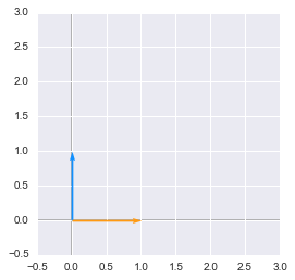
The unit vectors
to $i$ and $j$. You can notice that this matrix is special: it is diagonal. So it will only rescale our space. No rotation here. More precisely, it will rescale each dimension the same way because the diagonal values are identical. Let’s create the matrix $\bs$:
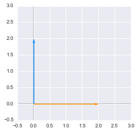
The transformed unit vectors: their lengths was multiplied by 2
As expected, we can see that the square corresponding to $i$ and $j$ didn’t rotate but the lengths of $i$ and $j$ have doubled.
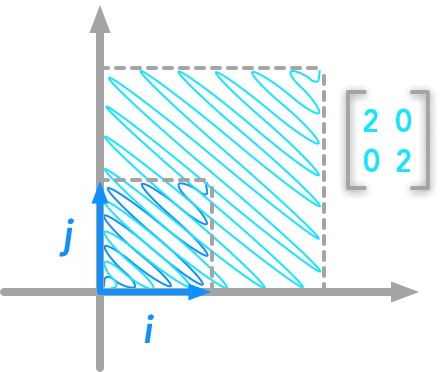
The unit square transformed by the matrix
We will now calculate the determinant of $\bs$ (you can go to the Wikipedia article for more details about the calculation of the determinant):
And yes, the transformation have multiplied the area of the unit square by 4. The lengths of $new_i$ and $new_j$ are $2$ (thus $2\cdot2=4$).
Example 2.
Let’s see now an example of negative determinant.
We will transform the unit square with the matrix:
Its determinant is $-4$:
The unit vectors transformed by the matrix with a negative determinant
We can see that the matrices with determinant $2$ and $-2$ modified the area of the unit square the same way.
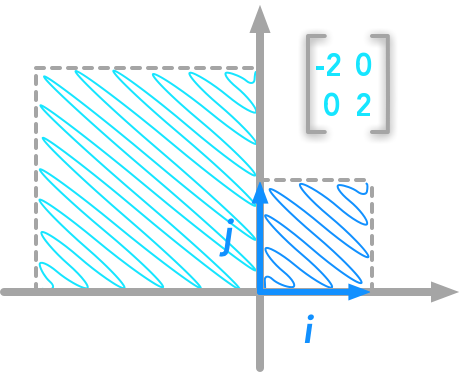
The unit square transformed by the matrix with a negative determinant
The absolute value of the determinant shows that, as in the first example, the area of the new square is 4 times the area of the unit square. But this time, it was not just a rescaling but also a transformation. It is not obvious with only the unit vectors so let’s transform some random points. We will use the matrix
that has a determinant equal to $-1$ for simplicity:
Since the determinant is $-1$, the area of the space will not be changed. However, since it is negative we will observe a transformation that we can’t obtain through rotation:
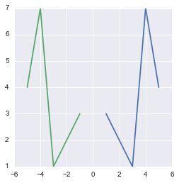
The transformation obtained with a negative determinant matrix is more than rescaling and rotating
You can see that the transformation mirrored the initial shape.
Conclusion
We have seen that the determinant of a matrix is a special value telling us a lot of things on the transformation corresponding to this matrix. Now hang on and go to the last chapter on the Principal Component Analysis (PCA).
References
Linear transformations
Numpy
Feel free to drop me an email or a comment. The syllabus of this series can be found in the introduction post. All the notebooks can be found on Github.
This content is part of a series following the chapter 2 on linear algebra from the Deep Learning Book by Goodfellow, I., Bengio, Y., and Courville, A. (2016). It aims to provide intuitions/drawings/python code on mathematical theories and is constructed as my understanding of these concepts. You can check the syllabus in the introduction post.
NumPy linalg.det – Compute the determinant of the given array

Hello and welcome to this tutorial on Numpy linalg.det. In this tutorial, we will be learning about the NumPy linalg.det() method and also seeing a lot of examples regarding the same. So let us begin!
What is numpy.linalg.det?
The numpy.linalg.det() method in NumPy is used to compute the determinant of a given square matrix.
If we have a 2×2 matrix of the form:
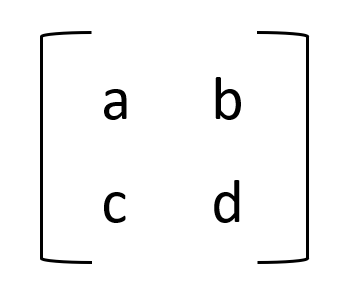
2×2 Array
Its determinant is calculated as:
alt=»2×2 Array Determinant» width=»283″ height=»157″ />2×2 Array Determinant
For a 3×3 matrix like
alt=»3×3 Array» width=»452″ height=»316″ />3×3 Array
The determinant is computed as:
alt=»3×3 Array Determinant» width=»561″ height=»61″ />3×3 Array Determinant
5 Numpy Functions with realistic Implementation
![]()
N umPy is a general-purpose array-processing package with some great mathematical functions to work with that could easily attract any math nerds and ML enthusiasts . Numpy provides a high-performance multidimensional array object, and lots of interesting APIs. Here are five numpy functions you should know. I have tried to mimic some realistic frames with these function so that each of them can make sense, at least at the time of introductory lessons. Most of the examples are related to linear and vector algebra. Even if you have basic understanding related to these topics you can continue with these article. I have tried here to put everything down in simple ways.
For more information related to Numpy APIs must visit the official site.
Disclaimer: The following blog is not only about coding rather it walks through the underlying mathematics of these functions.
Functions to be covered :
1. numpy.linalg.det
2. numpy.linalg.norm
3. numpy.dot
4. numpy.angle
5. numpy.linalg.solve
Function 1 : numpy.linalg.det
This numpy function can evaluate the determinant of a square matrix. For example:
for this ‘arr’ matrix the function will return the determinant of the matrix is -306.
Implementation: Area of triangle.
The area of triangle whose three coordinates are given say, x(3, 3, 1), y(-3, 2, -1) and z(8, 6, 3) can be measured using the following formula:
Here, each row represents the x-y-z components of a point in a given three dimensional space.
Explanation: Here, find_triangular_area takes three points with corresponding x-y-z components in lists, enclose these lists in a parent array and thus create a 3×3 matrix representing the triangle in three dimensional space. Then it calculate its determinant. Half of the determinant is the area of the given triangle. Return.
Function 2: numpy.linalg.norm
The function calculate the modulus of a given vector or a matrix.
Essentially the norm determines the magnitude of a vector or a square matrix. There are multiple types of norms for a vector and matrix. Some common norms are: 1-norm, 2-norm or Euclidean norm, positive infinity-norm, negative infinity-norm, Frobenius norm etc. For more information of numpy linalg.norm function see here.
The type 2-norm calculate the Euclidean distance of a given vector from the origin:
The numpy linalg.norm() function takes 4 arguments. Two are most useful:
x: Take vector or matrix as input and,
ord: Defines the type of norm. In case left blank, it calculates the 2-norm for vectors and Frobenius norm for matrix.
Implementation: Calculate distance between two points.
Explanation:
Here, in cal_distance function, both vectors are encoated in numpy array as np.linalg.norm() function only takes numpy array as argument. Then the difference between each vector passes to the norm() to calculate the Euclidean distance. Return.
Function 3: numpy.dot
This function returns the dot product of two vectors. Dot product defines how much of a vector is pointing towards the another vector. If the two vectors are pointing at the same direction then the resultant would be large positive scalar and if the two vectors pointing perpendicularly then the magnitude of the resultant will be zero and quite in the opposite direction will produce negative resultant. Mathematically it can be defined as:
Implementation: Find if two given vectors are perpendicular or not
Explanation:
The is_perpendicular function, takes the components of two vectors in two numpy arrays. calculate their dot product using numpy.dot() function. If the dot product of two vector is equal to zero then it returns True as two perpendicular vectors cancel out each other effect in that direction.
Function 4: numpy.angle
This function calculate the complex argument. Complex argument is essentially the angle between Real Axis and the line joining complex point (z) in the complex plane.
Let’s, find out the maths of complex argument. Say a complex number
where x is the “real” part and y is the “imaginary” part of the complex number z. Now any complex number can be represented as exponential form:
You can find more interesting explanation of Complex argument in Here.
Implementation: Calculating angle between two complex numbers
Explanation:
The find_cmplx_angle function, takes two complex numbers. The numbers must be encoated before passing to numpy.angle() method. The numpy.angle() method calculate the corresponding arguments of the complex numbers of the cmplx_list and return the result as numpy array to cmplx_angle . Then difference between the angle is calculated and Return.
Function 5: numpy.linalg.solve
This function does solve a linear matrix equation or system of linear equation. Consider the following system of equations, represent planes in a three dimensional space have a common point of intersection:
The equations can be rewritten as:
A general intuition is that the equations that are not parallel (considering three distinct planes in 3D or two lines in 2D space), the single point of intersection will satisfy all the equations and therefore represent the solution to the system.
The numpy.linalg.solve() function solves these equations by taking matrices out these equation which is look like following one:
You can find a good blog describing the whole process with example in here.
Implementation: Solve a linear system of equations
Explanation:
The solve_system wrapper function, takes all three coefficient vectors of the equations and wrap it in coefficient matrix (numpy array) and also dependent variables. Pass both array to numpy.linalg.solve() method. Return.
This article is enriched with the enormous articles and blogs of the following portals: