numpy.exp#
Calculate the exponential of all elements in the input array.
Parameters : x array_like
out ndarray, None, or tuple of ndarray and None, optional
A location into which the result is stored. If provided, it must have a shape that the inputs broadcast to. If not provided or None, a freshly-allocated array is returned. A tuple (possible only as a keyword argument) must have length equal to the number of outputs.
where array_like, optional
This condition is broadcast over the input. At locations where the condition is True, the out array will be set to the ufunc result. Elsewhere, the out array will retain its original value. Note that if an uninitialized out array is created via the default out=None , locations within it where the condition is False will remain uninitialized.
**kwargs
For other keyword-only arguments, see the ufunc docs .
Returns : out ndarray or scalar
Output array, element-wise exponential of x. This is a scalar if x is a scalar.
Calculate exp(x) — 1 for all elements in the array.
Calculate 2**x for all elements in the array.
The irrational number e is also known as Euler’s number. It is approximately 2.718281, and is the base of the natural logarithm, ln (this means that, if \(x = \ln y = \log_e y\) , then \(e^x = y\) . For real input, exp(x) is always positive.
For complex arguments, x = a + ib , we can write \(e^x = e^a e^
NumPy Exponential: Using the NumPy.exp() Function

In this tutorial, you’ll learn how to use the NumPy exponential function, np.exp(). The function raises the Euler’s constant, e , to a given power. Because Euler’s constant has many practical applications in science, math, and deep learning, being able to work with this function in meaningful ways is an asset for any Python user!
By the end of this tutorial, you’ll have learned:
- What the np.exp() function does
- How to apply the function to a single value and to NumPy arrays
- How to use the function to graph exponential arrays
Table of Contents
Understanding the np.exp() Function
The NumPy exp() function is used to calculate the exponential of all the elements in an array. This means that it raises the value of Euler’s constant, e , to the power all elements of an array, or a single element, passed into the function. Euler’s constant is roughly equal to 2.718 and has many practical applications such as calculating compound interest. To learn more about Euler’s constant in Python, check out my in-depth tutorial here.
The exponential function is commonly used in deep learning in the development of the sigmoid function. Let’s take a look at the function:
In most cases, you’ll see the function applied only with the x argument supplied. Let’s take a look at how we can run the function with a single value passed in:
The function call above is the same as calling e 1 . The real value of the function comes into play when its applied to entire arrays of numbers. This is what you’ll learn in the next section.
How to Apply the np.exp() Function to a 2-Dimensional Array
In this section, you’ll learn how to apply the np.exp() function an array of numbers. Applying the function to an array works the same as applying it to a scalar, only that we pass in an array. Because numpy works array-wise, the function is applied to each element in that array.
Let’s take a look at an example:
In the example above, we use the np.arange() function to create the values from 1 through 5. We then pass this array into the np.exp() function to process each item.
The function also works for multi-dimensional arrays, as shown in the next section.
Building basic functions with numpy
![]()
Numpy is the main package for scientific computing in Python. It is maintained by a large community (www.numpy.org). In this exercise you will learn several key numpy functions such as np.exp, np.log, and np.reshape. You will need to know how to use these functions for future assignments.
sigmoid function, np.exp()
Before using np.exp(), you will use math.exp() to implement the sigmoid function. You will then see why np.exp() is preferable to math.exp().
Exercise: Build a function that returns the sigmoid of a real number x. Use math.exp(x) for the exponential function.
Reminder: sigmoid(x)=11+e−xsigmoid(x)=11+e−x is sometimes also known as the logistic function. It is a non-linear function used not only in Machine Learning (Logistic Regression), but also in Deep Learning.
Sigmoid gradient
As you’ve seen in lecture, you will need to compute gradients to optimize loss functions using backpropagation. Let’s code your first gradient function.
Exercise: Implement the function sigmoid_grad() to compute the gradient of the sigmoid function with respect to its input x. The formula is:
You often code this function in two steps:
- Set s to be the sigmoid of x. You might find your sigmoid(x) function useful.
- Compute σ′(x)=s(1−s)σ′(x)=s(1−s)
Reshaping arrays
Two common numpy functions used in deep learning are np.shape and np.reshape().
- X.shape is used to get the shape (dimension) of a matrix/vector X.
- X.reshape(…) is used to reshape X into some other dimension.
For example, in computer science, an image is represented by a 3D array of shape (length,height,depth=3)(length,height,depth=3). However, when you read an image as the input of an algorithm you convert it to a vector of shape (length∗height∗3,1)(length∗height∗3,1). In other words, you “unroll”, or reshape, the 3D array into a 1D vector.
Normalizing rows
Another common technique we use in Machine Learning and Deep Learning is to normalize our data. It often leads to a better performance because gradient descent converges faster after normalization. Here, by normalization we mean changing x to x∥x∥x∥x∥ (dividing each row vector of x by its norm).
Note that you can divide matrices of different sizes and it works fine: this is called broadcasting and you’re going to learn about it in part 5.
Broadcasting and the softmax function
A very important concept to understand in numpy is “broadcasting”. It is very useful for performing mathematical operations between arrays of different shapes. For the full details on broadcasting, you can read the official broadcasting documentation.
Exercise: Implement a softmax function using numpy. You can think of softmax as a normalizing function used when your algorithm needs to classify two or more classes. You will learn more about softmax in the second course of this specialization.
Instructions:
- for x∈ℝ1×n, softmax(x)=softmax([x1x2…xn])=[ex1∑jexjex2∑jexj…exn∑jexj]for x∈R1×n, softmax(x)=softmax([x1x2…xn])=[ex1∑jexjex2∑jexj…exn∑jexj]
- for a matrix x∈ℝm×n, xij maps to the element in the ith row and jth column of x, thus we have: for a matrix x∈Rm×n, xij maps to the element in the ith row and jth column of x, thus we have:
- softmax(x)=softmaxx11x21⋮xm1x12x22⋮xm2x13x23⋮xm3……⋱…x1nx2n⋮xmn=ex11∑jex1jex21∑jex2j⋮exm1∑jexmjex12∑jex1jex22∑jex2j⋮exm2∑jexmjex13∑jex1jex23∑jex2j⋮exm3∑jexmj……⋱…ex1n∑jex1jex2n∑jex2j⋮exmn∑jexmj=softmax(first row of x)softmax(second row of x)…softmax(last row of x)softmax(x)=softmax[x11x12x13…x1nx21x22x23…x2n⋮⋮⋮⋱⋮xm1xm2xm3…xmn]=[ex11∑jex1jex12∑jex1jex13∑jex1j…ex1n∑jex1jex21∑jex2jex22∑jex2jex23∑jex2j…ex2n∑jex2j⋮⋮⋮⋱⋮exm1∑jexmjexm2∑jexmjexm3∑jexmj…exmn∑jexmj]=(softmax(first row of x)softmax(second row of x)…softmax(last row of x))
Note that later in the course, you’ll see “m” used to represent the “number of training examples”, and each training example is in its own column of the matrix.
Also, each feature will be in its own row (each row has data for the same feature).
Softmax should be performed for all features of each training example, so softmax would be performed on the columns (once we switch to that representation later in this course).
However, in this coding practice, we’re just focusing on getting familiar with Python, so we’re using the common math notation m×nm×n
where mm is the number of rows and nn is the number of columns.
Vectorization
In deep learning, you deal with very large datasets. Hence, a non-computationally-optimal function can become a huge bottleneck in your algorithm and can result in a model that takes ages to run. To make sure that your code is computationally efficient, you will use vectorization. For example, try to tell the difference between the following implementations of the dot/outer/elementwise product.
Implement the L1 and L2 loss functions
Exercise: Implement the numpy vectorized version of the L1 loss. You may find the function abs(x) (absolute value of x) useful.
NumPy exp – A Complete Guide

Hello and welcome to this tutorial on Numpy exp. In this tutorial, we will be learning about the NumPy exp() method and also seeing a lot of examples regarding the same. So let us begin!
What is NumPy exp?
The exp method in NumPy is a function that returns the exponential of all the elements of the input array. This means that it calculates e^x for each x in the input array. Here, e is the Euler’s constant and has a value of approximately 2.718281.
It can be said that np.exp(i) is approximately equal to e**i, where ‘**’ is the power operator. We will see the examples for this function in the upcoming section of this tutorial.
Syntax of NumPy exp method
| Parameter | Description | Required/Optional |
| x | Input array/value. | Required |
| out | An alternative output array in which to place the result. By default, a new array is created. | Optional |
| where | Takes an array-like object. At locations where it is True, the out array will be set to the ufunc result. Elsewhere, the out array will retain its original value. | Optional |
| **kwargs | For other keyword-only arguments | Optional |
Returns: An array containing the element-wise exponential of x. If x is a scalar, then the result is also a scalar.
Using the Numpy exp() method
Let’s check out how to use the numpy exp method through different examples.
1. Exponential of a scalar value using numpy exp()
Output:
The answer is calculated as e^6 i.e. (2.718281)^6 = 403.4287934927351.
Output:
In this case, since a is a negative number, the exponential of a is (e)^(-6) i.e. 1/(e)^6 = 1/(2.718281)^6 = 0.0024787521766663585.
2. Exponential of a 1-dimensional array using numpy exp()
Output:
Here, the result array contains the exponential of e for each value in the input array. That is, the and contains the values, e^0, e^3, e^-2 and e^1 in order of the input values.
3. Exponential of a 2-dimensional array using numpy exp()
Output:
Similar to the above example, the resulting array contains an exponential of e for each value in the input array in order.
4. Plotting the graph of np.exp() using numpy exp()
Let us now plot the graph of the np.exp() function against some input values using the Matplotlib library in Python.
Output:
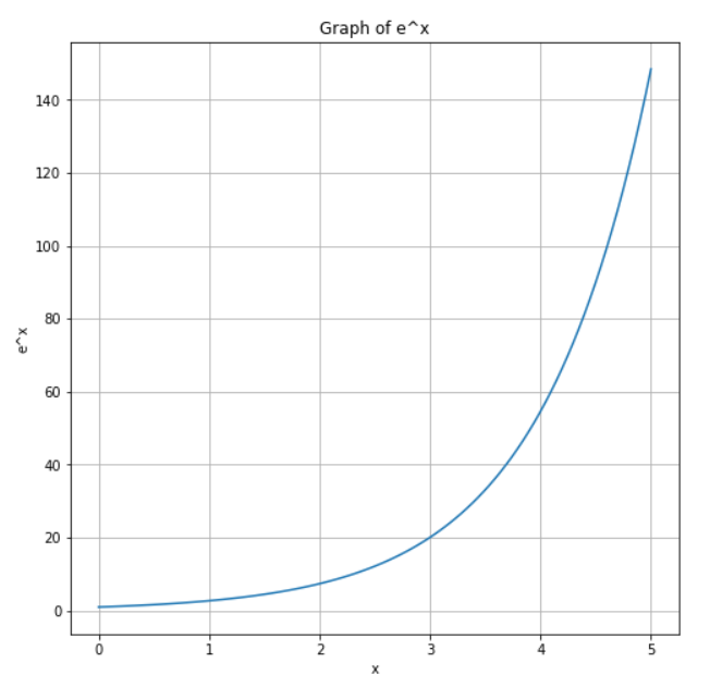
Graph Of Exponential
In this example, we have created an evenly spaced array of numbers (x) from 0 to 5 having 100 values in total. Then this array is passed to the np.exp() function and stored in the result in y. At last, we plot the graph of y v/s x and get the above plot as the result.
Summary
That’s all! In this tutorial, we learned about the Numpy exp method and practiced different types of examples using the same. If you want to learn more about NumPy, feel free to go through our NumPy tutorials.