Hyperparameter tuning#
In the previous section, we did not discuss the parameters of random forest and gradient-boosting. However, there are a couple of things to keep in mind when setting these.
This notebook gives crucial information regarding how to set the hyperparameters of both random forest and gradient boosting decision tree models.
For the sake of clarity, no cross-validation will be used to estimate the variability of the testing error. We are only showing the effect of the parameters on the validation set of what should be the inner loop of a nested cross-validation.
We will start by loading the california housing dataset.
Random forest#
The main parameter to select in random forest is the n_estimators parameter. In general, the more trees in the forest, the better the generalization performance will be. However, it will slow down the fitting and prediction time. The goal is to balance computing time and generalization performance when setting the number of estimators. Here, we fix n_estimators=100 , which is already the default value.
Tuning the n_estimators for random forests generally result in a waste of computer power. We just need to ensure that it is large enough so that doubling its value does not lead to a significant improvement of the validation error.
Instead, we can tune the hyperparameter max_features , which controls the size of the random subset of features to consider when looking for the best split when growing the trees: smaller values for max_features will lead to more random trees with hopefully more uncorrelated prediction errors. However if max_features is too small, predictions can be too random, even after averaging with the trees in the ensemble.
If max_features is set to None , then this is equivalent to setting max_features=n_features which means that the only source of randomness in the random forest is the bagging procedure.
We can also tune the different parameters that control the depth of each tree in the forest. Two parameters are important for this: max_depth and max_leaf_nodes . They differ in the way they control the tree structure. Indeed, max_depth will enforce to have a more symmetric tree, while max_leaf_nodes does not impose such constraint. If max_leaf_nodes=None then the number of leaf nodes is unlimited.
The hyperparameter min_samples_leaf controls the minimum number of samples required to be at a leaf node. This means that a split point (at any depth) is only done if it leaves at least min_samples_leaf training samples in each of the left and right branches. A small value for min_samples_leaf means that some samples can become isolated when a tree is deep, promoting overfitting. A large value would prevent deep trees, which can lead to underfitting.
Be aware that with random forest, trees are expected to be deep since we are seeking to overfit each tree on each bootstrap sample. Overfitting is mitigated when combining the trees altogether, whereas assembling underfitted trees (i.e. shallow trees) might also lead to an underfitted forest.
| param_max_features | param_max_leaf_nodes | param_min_samples_leaf | mean_test_error | std_test_error | |
|---|---|---|---|---|---|
| 3 | 2 | None | 2 | 33.994711 | 0.538897 |
| 0 | 2 | 1000 | 10 | 36.828591 | 0.432680 |
| 7 | None | None | 20 | 37.321178 | 0.441737 |
| 4 | 5 | 100 | 2 | 40.041925 | 0.647538 |
| 8 | None | 100 | 10 | 40.364790 | 0.743403 |
| 6 | None | 1000 | 50 | 40.744152 | 0.443388 |
| 9 | 1 | 100 | 2 | 49.719213 | 0.670644 |
| 2 | 1 | 100 | 1 | 50.106131 | 0.638342 |
| 5 | 1 | None | 100 | 54.807478 | 0.910029 |
| 1 | 3 | 10 | 10 | 54.932381 | 0.846035 |
We can observe in our search that we are required to have a large number of max_leaf_nodes and thus deep trees. This parameter seems particularly impactful with respect to the other tuning parameters, but large values of min_samples_leaf seem to reduce the performance of the model.
In practice, more iterations of random search would be necessary to precisely assert the role of each parameters. Using n_iter=10 is good enough to quickly inspect the hyperparameter combinations that yield models that work well enough without spending too much computational resources. Feel free to try more interations on your own.
Once the RandomizedSearchCV has found the best set of hyperparameters, it uses them to refit the model using the full training set. To estimate the generalization performance of the best model it suffices to call .score on the unseen data.
Gradient-boosting decision trees#
For gradient-boosting, parameters are coupled, so we cannot set the parameters one after the other anymore. The important parameters are n_estimators , learning_rate , and max_depth or max_leaf_nodes (as previously discussed random forest).
Let’s first discuss the max_depth (or max_leaf_nodes ) parameter. We saw in the section on gradient-boosting that the algorithm fits the error of the previous tree in the ensemble. Thus, fitting fully grown trees would be detrimental. Indeed, the first tree of the ensemble would perfectly fit (overfit) the data and thus no subsequent tree would be required, since there would be no residuals. Therefore, the tree used in gradient-boosting should have a low depth, typically between 3 to 8 levels, or few leaves ( \(2^3=8\) to \(2^8=256\) ). Having very weak learners at each step will help reducing overfitting.
With this consideration in mind, the deeper the trees, the faster the residuals will be corrected and less learners are required. Therefore, n_estimators should be increased if max_depth is lower.
Finally, we have overlooked the impact of the learning_rate parameter until now. When fitting the residuals, we would like the tree to try to correct all possible errors or only a fraction of them. The learning-rate allows you to control this behaviour. A small learning-rate value would only correct the residuals of very few samples. If a large learning-rate is set (e.g., 1), we would fit the residuals of all samples. So, with a very low learning-rate, we will need more estimators to correct the overall error. However, a too large learning-rate tends to obtain an overfitted ensemble, similar to having a too large tree depth.
| param_n_estimators | param_max_leaf_nodes | param_learning_rate | mean_test_error | std_test_error | |
|---|---|---|---|---|---|
| 1 | 200 | 20 | 0.160519 | 33.905197 | 0.433738 |
| 12 | 200 | 50 | 0.110585 | 34.793012 | 0.292925 |
| 17 | 500 | 5 | 0.771785 | 34.822201 | 0.517495 |
| 10 | 200 | 20 | 0.109889 | 35.004927 | 0.376778 |
| 6 | 500 | 100 | 0.709894 | 35.465560 | 0.306254 |
| 18 | 10 | 5 | 0.637819 | 42.535730 | 0.338066 |
| 3 | 500 | 2 | 0.07502 | 43.457866 | 0.704599 |
| 4 | 100 | 5 | 0.0351 | 46.558900 | 0.578629 |
| 19 | 5 | 20 | 0.202432 | 61.387176 | 0.610988 |
| 8 | 5 | 2 | 0.462636 | 65.114017 | 0.846987 |
| 9 | 10 | 5 | 0.088556 | 66.243538 | 0.720131 |
| 15 | 50 | 100 | 0.010904 | 71.847050 | 0.683326 |
| 5 | 2 | 2 | 0.421054 | 74.384704 | 0.791104 |
| 2 | 5 | 100 | 0.070357 | 77.007841 | 0.789595 |
| 16 | 2 | 50 | 0.167568 | 77.131005 | 0.850380 |
| 11 | 1 | 5 | 0.190477 | 82.819015 | 0.976351 |
| 13 | 5 | 20 | 0.033815 | 83.765509 | 0.974672 |
| 0 | 1 | 100 | 0.125207 | 85.363288 | 1.040982 |
| 14 | 1 | 10 | 0.081715 | 87.373374 | 1.071555 |
| 7 | 1 | 20 | 0.014937 | 90.531295 | 1.113892 |
Here, we tune the n_estimators but be aware that is better to use early_stopping as done in the Exercise M6.04.
In this search, we see that the learning_rate is required to be large enough, i.e. > 0.1. We also observe that for the best ranked models, having a smaller learning_rate , will require more trees or a larger number of leaves for each tree. However, it is particularly difficult to draw more detailed conclusions since the best value of an hyperparameter depends on the other hyperparameter values.
Now we estimate the generalization performance of the best model using the test set.
The mean test score in the held-out test set is slightly better than the score of the best model. The reason is that the final model is refitted on the whole training set and therefore, on more data than the cross-validated models of the grid search procedure.
In Depth: Parameter tuning for Random Forest

In this post we will explore the most important parameters of Random Forest and how they impact our model in term of overfitting and underfitting.
A random forest is a meta estimator that fits a number of decision tree classifiers on various sub-samples of the dataset and use averaging to improve the predictive accuracy and control over-fitting.
We will use the Titanic Data from kaggle. For the sake of this post, we will perform as little feature engineering as possible as it is not the purpose of this post.
Load train data
Check for missing values
We will remove ‘Cabin’, ‘Name’ and ‘Ticket’ columns as they require some processing to extract useful features
Fill the missing age values by the mean value
Fill the missing ‘Embarked’ values by the most frequent value
‘Pclass’ is a categorical feature so we convert its values to strings
Let’s perform a basic one hot encoding of categorical features
For testing, we choose to split our data to 75% train and 25% for test
Let’s first fit a random forest with default parameters to get a baseline idea of the performance
We will use AUC (Area Under Curve) as the evaluation metric. Our target value is binary so it’s a binary classification problem. AUC is a good way for evaluation for this type of problems.
N_estimators
n_estimators represents the number of trees in the forest. Usually the higher the number of trees the better to learn the data. However, adding a lot of trees can slow down the training process considerably, therefore we do a parameter search to find the sweet spot.
We can see that for our data, we can stop at 32 trees as increasing the number of trees decreases the test performance.
max_depth
max_depth represents the depth of each tree in the forest. The deeper the tree, the more splits it has and it captures more information about the data. We fit each decision tree with depths ranging from 1 to 32 and plot the training and test errors.
We see that our model overfits for large depth values. The trees perfectly predicts all of the train data, however, it fails to generalize the findings for new data
min_samples_split
min_samples_split represents the minimum number of samples required to split an internal node. This can vary between considering at least one sample at each node to considering all of the samples at each node. When we increase this parameter, each tree in the forest becomes more constrained as it has to consider more samples at each node. Here we will vary the parameter from 10% to 100% of the samples
We can clearly see that when we require all of the samples at each node, the model cannot learn enough about the data. This is an underfitting case.
min_samples_leaf
min_samples_leaf is The minimum number of samples required to be at a leaf node. This parameter is similar to min_samples_splits, however, this describe the minimum number of samples of samples at the leafs, the base of the tree.
Same conclusion as to previous parameter. Increasing this value can cause underfitting.
max_features
max_features represents the number of features to consider when looking for the best split.
This is also an overfitting case. It’s unexpected to get overfitting for all values of max_features. However, according to sklearn documentation for random forest, the search for a split does not stop until at least one valid partition of the node samples is found, even if it requires to effectively inspect more than max_features features.
The inDepth series investigates how model parameters affect performance in term of overfitting and underfitting. This is the second post in the series. You can check the inDepth Decision Tree or wait for the next post about Gradient Boosting.
sklearn.ensemble .RandomForestClassifier
A random forest is a meta estimator that fits a number of decision tree classifiers on various sub-samples of the dataset and uses averaging to improve the predictive accuracy and control over-fitting. The sub-sample size is controlled with the max_samples parameter if bootstrap=True (default), otherwise the whole dataset is used to build each tree.
Read more in the User Guide .
Parameters : n_estimators int, default=100
The number of trees in the forest.
Changed in version 0.22: The default value of n_estimators changed from 10 to 100 in 0.22.
The function to measure the quality of a split. Supported criteria are “gini” for the Gini impurity and “log_loss” and “entropy” both for the Shannon information gain, see Mathematical formulation . Note: This parameter is tree-specific.
max_depth int, default=None
The maximum depth of the tree. If None, then nodes are expanded until all leaves are pure or until all leaves contain less than min_samples_split samples.
min_samples_split int or float, default=2
The minimum number of samples required to split an internal node:
If int, then consider min_samples_split as the minimum number.
If float, then min_samples_split is a fraction and ceil(min_samples_split * n_samples) are the minimum number of samples for each split.
Changed in version 0.18: Added float values for fractions.
The minimum number of samples required to be at a leaf node. A split point at any depth will only be considered if it leaves at least min_samples_leaf training samples in each of the left and right branches. This may have the effect of smoothing the model, especially in regression.
If int, then consider min_samples_leaf as the minimum number.
If float, then min_samples_leaf is a fraction and ceil(min_samples_leaf * n_samples) are the minimum number of samples for each node.
Changed in version 0.18: Added float values for fractions.
The minimum weighted fraction of the sum total of weights (of all the input samples) required to be at a leaf node. Samples have equal weight when sample_weight is not provided.
max_features <“sqrt”, “log2”, None>, int or float, default=”sqrt”
The number of features to consider when looking for the best split:
If int, then consider max_features features at each split.
If float, then max_features is a fraction and max(1, int(max_features * n_features_in_)) features are considered at each split.
If “auto”, then max_features=sqrt(n_features) .
If “sqrt”, then max_features=sqrt(n_features) .
If “log2”, then max_features=log2(n_features) .
If None, then max_features=n_features .
Changed in version 1.1: The default of max_features changed from "auto" to "sqrt" .
Deprecated since version 1.1: The "auto" option was deprecated in 1.1 and will be removed in 1.3.
Note: the search for a split does not stop until at least one valid partition of the node samples is found, even if it requires to effectively inspect more than max_features features.
max_leaf_nodes int, default=None
Grow trees with max_leaf_nodes in best-first fashion. Best nodes are defined as relative reduction in impurity. If None then unlimited number of leaf nodes.
min_impurity_decrease float, default=0.0
A node will be split if this split induces a decrease of the impurity greater than or equal to this value.
The weighted impurity decrease equation is the following:
where N is the total number of samples, N_t is the number of samples at the current node, N_t_L is the number of samples in the left child, and N_t_R is the number of samples in the right child.
N , N_t , N_t_R and N_t_L all refer to the weighted sum, if sample_weight is passed.
New in version 0.19.
Whether bootstrap samples are used when building trees. If False, the whole dataset is used to build each tree.
oob_score bool, default=False
Whether to use out-of-bag samples to estimate the generalization score. Only available if bootstrap=True.
n_jobs int, default=None
The number of jobs to run in parallel. fit , predict , decision_path and apply are all parallelized over the trees. None means 1 unless in a joblib.parallel_backend context. -1 means using all processors. See Glossary for more details.
random_state int, RandomState instance or None, default=None
Controls both the randomness of the bootstrapping of the samples used when building trees (if bootstrap=True ) and the sampling of the features to consider when looking for the best split at each node (if max_features < n_features ). See Glossary for details.
verbose int, default=0
Controls the verbosity when fitting and predicting.
warm_start bool, default=False
When set to True , reuse the solution of the previous call to fit and add more estimators to the ensemble, otherwise, just fit a whole new forest. See Glossary and Fitting additional weak-learners for details.
class_weight <“balanced”, “balanced_subsample”>, dict or list of dicts, default=None
Weights associated with classes in the form
Note that for multioutput (including multilabel) weights should be defined for each class of every column in its own dict. For example, for four-class multilabel classification weights should be [<0: 1, 1: 1>, <0: 1, 1: 5>, <0: 1, 1: 1>, <0: 1, 1: 1>] instead of [<1:1>, <2:5>, <3:1>, <4:1>].
The “balanced” mode uses the values of y to automatically adjust weights inversely proportional to class frequencies in the input data as n_samples / (n_classes * np.bincount(y))
The “balanced_subsample” mode is the same as “balanced” except that weights are computed based on the bootstrap sample for every tree grown.
For multi-output, the weights of each column of y will be multiplied.
Note that these weights will be multiplied with sample_weight (passed through the fit method) if sample_weight is specified.
ccp_alpha non-negative float, default=0.0
Complexity parameter used for Minimal Cost-Complexity Pruning. The subtree with the largest cost complexity that is smaller than ccp_alpha will be chosen. By default, no pruning is performed. See Minimal Cost-Complexity Pruning for details.
New in version 0.22.
If bootstrap is True, the number of samples to draw from X to train each base estimator.
If None (default), then draw X.shape[0] samples.
If int, then draw max_samples samples.
If float, then draw max_samples * X.shape[0] samples. Thus, max_samples should be in the interval (0.0, 1.0] .
New in version 0.22.
The child estimator template used to create the collection of fitted sub-estimators.
New in version 1.2: base_estimator_ was renamed to estimator_ .
Estimator used to grow the ensemble.
estimators_ list of DecisionTreeClassifier
The collection of fitted sub-estimators.
classes_ ndarray of shape (n_classes,) or a list of such arrays
The classes labels (single output problem), or a list of arrays of class labels (multi-output problem).
n_classes_ int or list
The number of classes (single output problem), or a list containing the number of classes for each output (multi-output problem).
n_features_in_ int
Number of features seen during fit .
New in version 0.24.
Names of features seen during fit . Defined only when X has feature names that are all strings.
New in version 1.0.
The number of outputs when fit is performed.
feature_importances_ ndarray of shape (n_features,)
The impurity-based feature importances.
oob_score_ float
Score of the training dataset obtained using an out-of-bag estimate. This attribute exists only when oob_score is True.
oob_decision_function_ ndarray of shape (n_samples, n_classes) or (n_samples, n_classes, n_outputs)
Decision function computed with out-of-bag estimate on the training set. If n_estimators is small it might be possible that a data point was never left out during the bootstrap. In this case, oob_decision_function_ might contain NaN. This attribute exists only when oob_score is True.
A decision tree classifier.
Ensemble of extremely randomized tree classifiers.
The default values for the parameters controlling the size of the trees (e.g. max_depth , min_samples_leaf , etc.) lead to fully grown and unpruned trees which can potentially be very large on some data sets. To reduce memory consumption, the complexity and size of the trees should be controlled by setting those parameter values.
The features are always randomly permuted at each split. Therefore, the best found split may vary, even with the same training data, max_features=n_features and bootstrap=False , if the improvement of the criterion is identical for several splits enumerated during the search of the best split. To obtain a deterministic behaviour during fitting, random_state has to be fixed.
Random Forest, метод главных компонент и оптимизация гиперпараметров: пример решения задачи классификации на Python
У специалистов по обработке и анализу данных есть множество средств для создания классификационных моделей. Один из самых популярных и надёжных методов разработки таких моделей заключается в использовании алгоритма «случайный лес» (Random Forest, RF). Для того чтобы попытаться улучшить показатели модели, построенной с использованием алгоритма RF, можно воспользоваться оптимизацией гиперпараметров модели (Hyperparameter Tuning, HT).

Кроме того, распространён подход, в соответствии с которым данные, перед их передачей в модель, обрабатывают с помощью метода главных компонент (Principal Component Analysis, PCA). Но стоит ли вообще этим пользоваться? Разве основная цель алгоритма RF заключается не в том, чтобы помочь аналитику интерпретировать важность признаков?
Да, применение алгоритма PCA может привести к небольшому усложнению интерпретации каждого «признака» при анализе «важности признаков» RF-модели. Однако алгоритм PCA производит уменьшение размерности пространства признаков, что может привести к уменьшению количества признаков, которые нужно обработать RF-моделью. Обратите внимание на то, что объёмность вычислений — это один из основных минусов алгоритма «случайный лес» (то есть — выполнение модели может занять немало времени). Применение алгоритма PCA может стать весьма важной частью моделирования, особенно в тех случаях, когда работают с сотнями или даже с тысячами признаков. В результате, если самое важное — это просто создать наиболее эффективную модель, и при этом можно пожертвовать точностью определения важности признаков, тогда PCA, вполне возможно, стоит попробовать.
Теперь — к делу. Мы будем работать с набором данных по раку груди — Scikit-learn «breast cancer». Мы создадим три модели и сравним их эффективность. А именно, речь идёт о следующих моделях:
- Базовая модель, основанная на алгоритме RF (будем сокращённо называть эту модель RF).
- Та же модель, что и №1, но такая, в которой применяется уменьшение размерности пространства признаков с помощью метода главных компонент (RF + PCA).
- Такая же модель, как и №2, но построенная с применением оптимизации гиперпараметров (RF + PCA + HT).
1. Импорт данных
Для начала загрузим данные и создадим датафрейм Pandas. Так как мы пользуемся предварительно очищенным «игрушечным» набором данных из Scikit-learn, то после этого мы уже сможем приступить к процессу моделирования. Но даже при использовании подобных данных рекомендуется всегда начинать работу, проведя предварительный анализ данных с использованием следующих команд, применяемых к датафрейму ( df ):
- df.head() — чтобы взглянуть на новый датафрейм и понять, выглядит ли он так, как ожидается.
- df.info() — чтобы выяснить особенности типов данных и содержимого столбцов. Возможно, перед продолжением работы понадобится произвести преобразование типов данных.
- df.isna() — чтобы убедиться в том, что в данных нет значений NaN . Соответствующие значения, если они есть, может понадобиться как-то обработать, или, если нужно, может понадобиться убрать целые строки из датафрейма.
- df.describe() — чтобы выяснить минимальные, максимальные, средние значения показателей в столбцах, чтобы узнать показатели среднеквадратического и вероятного отклонения по столбцам.

Фрагмент датафрейма с данными по раку груди. Каждая строка содержит результаты наблюдений за пациентом. Последний столбец, cancer, содержит целевую переменную, которую мы пытаемся предсказать. 0 означает «отсутствие заболевания». 1 — «наличие заболевания»
2. Разделение набора данных на учебные и проверочные данные
Теперь разделим данные с использованием функции Scikit-learn train_test_split . Мы хотим дать модели как можно больше учебных данных. Однако нужно, чтобы в нашем распоряжении было бы достаточно данных для проверки модели. В целом можно сказать, что, по мере роста количества строк в наборе данных, растёт и объём данных, которые можно рассматривать в качестве учебных.
Например, если есть миллионы строк, можно разделить набор, выделив 90% строк на учебные данные и 10% — на проверочные. Но исследуемый набор данных содержит лишь 569 строк. А это — не так уж и много для тренировки и проверки модели. В результате для того, чтобы быть справедливыми по отношению к учебным и проверочным данным, мы разделим набор на две равные части — 50% — учебные данные и 50% — проверочные. Мы устанавливаем stratify=y для обеспечения того, чтобы и в учебном, и в проверочном наборах данных присутствовало бы то же соотношение 0 и 1, что и в исходном наборе данных.
3. Масштабирование данных
Прежде чем приступать к моделированию, нужно выполнить «центровку» и «стандартизацию» данных путём их масштабирования. Масштабирование выполняется из-за того, что разные величины выражены в разных единицах измерения. Эта процедура позволяет организовать «честную схватку» между признаками при определении их важности. Кроме того, мы конвертируем y_train из типа данных Pandas Series в массив NumPy для того чтобы позже модель смогла бы работать с соответствующими целевыми показателями.
4. Обучение базовой модели (модель №1, RF)
Сейчас создадим модель №1. В ней, напомним, применяется только алгоритм Random Forest. Она использует все признаки и настроена с использованием значений, задаваемых по умолчанию (подробности об этих настройках можно найти в документации к sklearn.ensemble.RandomForestClassifier). Сначала инициализируем модель. После этого обучим её на масштабированных данных. Точность модели можно измерить на учебных данных:
Если нам интересно узнать о том, какие признаки являются самыми важными для RF-модели в деле предсказания рака груди, мы можем визуализировать и квантифицировать показатели важности признаков, обратившись к атрибуту feature_importances_ :
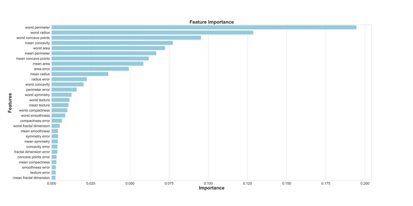
Визуализация «важности» признаков
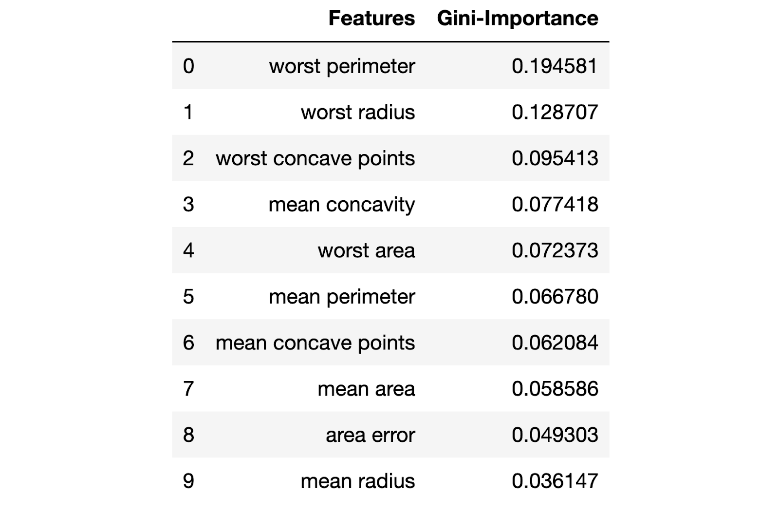
Показатели важности признаков
5. Метод главных компонент
Теперь зададимся вопросом о том, как можно улучшить базовую RF-модель. С использованием методики снижения размерности пространства признаков можно представить исходный набор данных через меньшее количество переменных и при этом снизить объём вычислительных ресурсов, необходимых для обеспечения работы модели. Используя PCA, можно изучить кумулятивную выборочную дисперсию этих признаков для того чтобы понять то, какие признаки объясняют большую часть дисперсии в данных.
Инициализируем объект PCA ( pca_test ), указывая количество компонент (признаков), которые нужно рассмотреть. Мы устанавливаем этот показатель в 30 для того чтобы увидеть объяснённую дисперсию всех сгенерированных компонент до того, как примем решение о том, сколько компонент нам понадобится. Затем передаём в pca_test масштабированные данные X_train , пользуясь методом pca_test.fit() . После этого визуализируем данные.
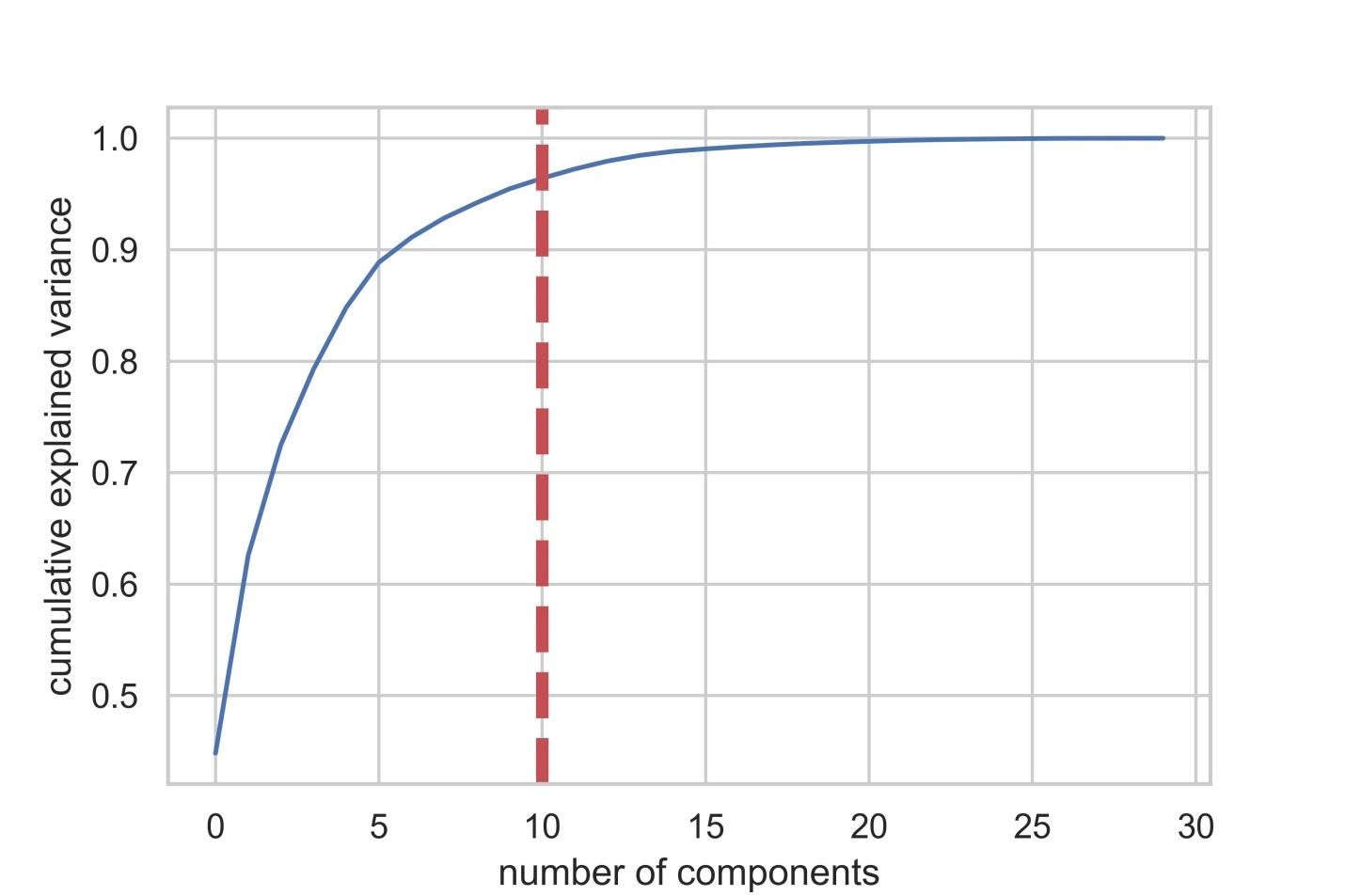
После того, как число используемых компонент превышает 10, рост их количества не очень сильно повышает объяснённую дисперсию
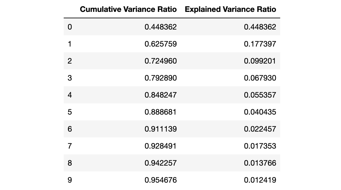
Этот датафрейм содержит такие показатели, как Cumulative Variance Ratio (кумулятивный размер объяснённой дисперсии данных) и Explained Variance Ratio (вклад каждой компоненты в общий объём объяснённой дисперсии)
Если взглянуть на вышеприведённый датафрейм, то окажется, что использование PCA для перехода от 30 переменных к 10 компонентам позволяет объяснить 95% дисперсии данных. Другие 20 компонент объясняют менее 5% дисперсии, а это значит, что от них мы можем отказаться. Следуя этой логике, воспользуемся PCA для уменьшения числа компонент с 30 до 10 для X_train и X_test . Запишем эти искусственно созданные наборы данных «пониженной размерности» в X_train_scaled_pca и в X_test_scaled_pca .
Каждая компонента — это линейная комбинация исходных переменных с соответствующими «весами». Мы можем видеть эти «веса» для каждой компоненты, создав датафрейм.
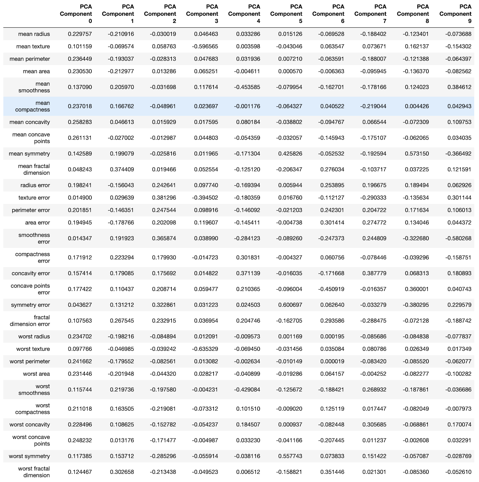
Датафрейм со сведениями по компонентам
6. Обучение базовой RF-модели после применения к данным метода главных компонент (модель №2, RF + PCA)
Теперь мы можем передать в ещё одну базовую RF-модель данные X_train_scaled_pca и y_train и можем узнать о том, есть ли улучшения в точности предсказаний, выдаваемых моделью.
Модели сравним ниже.
7. Оптимизация гиперпараметров. Раунд 1: RandomizedSearchCV
После обработки данных с использованием метода главных компонент можно попытаться воспользоваться оптимизацией гиперпараметров модели для того чтобы улучшить качество предсказаний, выдаваемых RF-моделью. Гиперпараметры можно рассматривать как что-то вроде «настроек» модели. Настройки, которые отлично подходят для одного набора данных, для другого не подойдут — поэтому и нужно заниматься их оптимизацией.
Начать можно с алгоритма RandomizedSearchCV, который позволяет довольно грубо исследовать широкие диапазоны значений. Описания всех гиперпараметров для RF-моделей можно найти здесь.
В ходе работы мы генерируем сущность param_dist , содержащую, для каждого гиперпараметра, диапазон значений, которые нужно испытать. Далее, мы инициализируем объект rs с помощью функции RandomizedSearchCV() , передавая ей RF-модель, param_dist , число итераций и число кросс-валидаций, которые нужно выполнить.
Гиперпараметр verbose позволяет управлять объёмом информации, который выводится моделью в ходе её работы (наподобие вывода сведений в процессе обучения модели). Гиперпараметр n_jobs позволяет указывать то, сколько процессорных ядер нужно использовать для обеспечения работы модели. Установка n_jobs в значение -1 приведёт к более быстрой работе модели, так как при этом будут использоваться все ядра процессора.
Мы будем заниматься подбором следующих гиперпараметров:
- n_estimators — число «деревьев» в «случайном лесу».
- max_features — число признаков для выбора расщепления.
- max_depth — максимальная глубина деревьев.
- min_samples_split — минимальное число объектов, необходимое для того, чтобы узел дерева мог бы расщепиться.
- min_samples_leaf — минимальное число объектов в листьях.
- bootstrap — использование для построения деревьев подвыборки с возвращением.
При значениях параметров n_iter = 100 и cv = 3 , мы создали 300 RF-моделей, случайно выбирая комбинации представленных выше гиперпараметров. Мы можем обратиться к атрибуту best_params_ для получения сведений о наборе параметров, позволяющем создать самую лучшую модель. Но на данной стадии это может не дать нам наиболее интересных данных о диапазонах параметров, которые стоит изучить на следующем раунде оптимизации. Для того чтобы выяснить то, в каком диапазоне значений стоит продолжать поиск, мы легко можем получить датафрейм, содержащий результаты работы алгоритма RandomizedSearchCV.
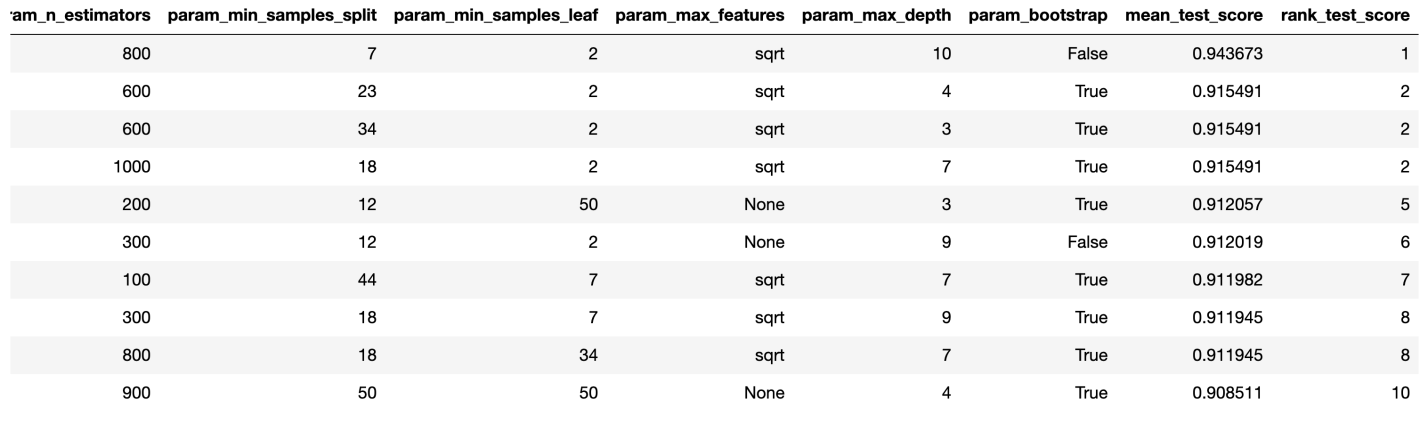
Результаты работы алгоритма RandomizedSearchCV
Теперь создадим столбчатые графики, на которых, по оси Х, расположены значения гиперпараметров, а по оси Y — средние значения, показываемые моделями. Это позволит понять то, какие значения гиперпараметров, в среднем, лучше всего себя показывают.
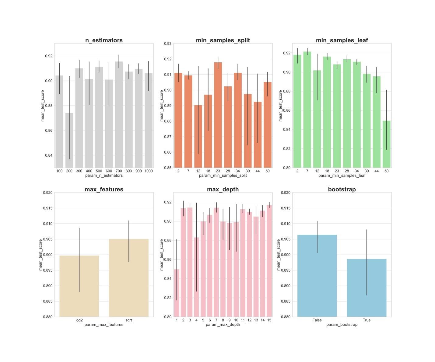
Анализ значений гиперпараметров
Если проанализировать вышеприведённые графики, то можно заметить некоторые интересные вещи, говорящие о том, как, в среднем, каждое значение гиперпараметра влияет на модель.
- n_estimators : значения 300, 500, 700, видимо, показывают наилучшие средние результаты.
- min_samples_split : маленькие значения, вроде 2 и 7, как кажется, показывают наилучшие результаты. Хорошо выглядит и значение 23. Можно исследовать несколько значений этого гиперпараметра, превышающих 2, а также — несколько значений около 23.
- min_samples_leaf : возникает такое ощущение, что маленькие значения этого гиперпараметра дают более высокие результаты. А это значит, что мы можем испытать значения между 2 и 7.
- max_features : вариант sqrt даёт самый высокий средний результат.
- max_depth : тут чёткой зависимости между значением гиперпараметра и результатом работы модели не видно, но есть ощущение, что значения 2, 3, 7, 11, 15 выглядят неплохо.
- bootstrap : значение False показывает наилучший средний результат.
8. Оптимизация гиперпараметров. Раунд 2: GridSearchCV (окончательная подготовка параметров для модели №3, RF + PCA + HT)
После применения алгоритма RandomizedSearchCV воспользуемся алгоритмом GridSearchCV для проведения более точного поиска наилучшей комбинации гиперпараметров. Здесь исследуются те же гиперпараметры, но теперь мы применяем более «обстоятельный» поиск их наилучшей комбинации. При использовании алгоритма GridSearchCV исследуется каждая комбинация гиперпараметров. Это требует гораздо больших вычислительных ресурсов, чем использование алгоритма RandomizedSearchCV, когда мы самостоятельно задаём число итераций поиска. Например, исследование 10 значений для каждого из 6 гиперпараметров с кросс-валидацией по 3 блокам потребует 10⁶ x 3, или 3000000 сеансов обучения модели. Именно поэтому мы и используем алгоритм GridSearchCV после того, как, применив RandomizedSearchCV, сузили диапазоны значений исследуемых параметров.
Итак, используя то, что мы выяснили с помощью RandomizedSearchCV, исследуем значения гиперпараметров, которые лучше всего себя показали:
Здесь мы применяем кросс-валидацию по 3 блокам для 540 (3 x 1 x 5 x 6 x 6 x 1) сеансов обучения модели, что даёт 1620 сеансов обучения модели. И уже теперь, после того, как мы воспользовались RandomizedSearchCV и GridSearchCV, мы можем обратиться к атрибуту best_params_ для того чтобы узнать о том, какие значения гиперпараметров позволяют модели наилучшим образом работать с исследуемым набором данных (эти значения можно видеть в нижней части предыдущего блока кода). Эти параметры используются при создании модели №3.
9. Оценка качества работы моделей на проверочных данных
Теперь можно оценить созданные модели на проверочных данных. А именно, речь идёт о тех трёх моделях, описанных в самом начале материала.
Проверим эти модели:
Создадим матрицы ошибок для моделей и узнаем о том, как хорошо каждая из них способна предсказывать рак груди:
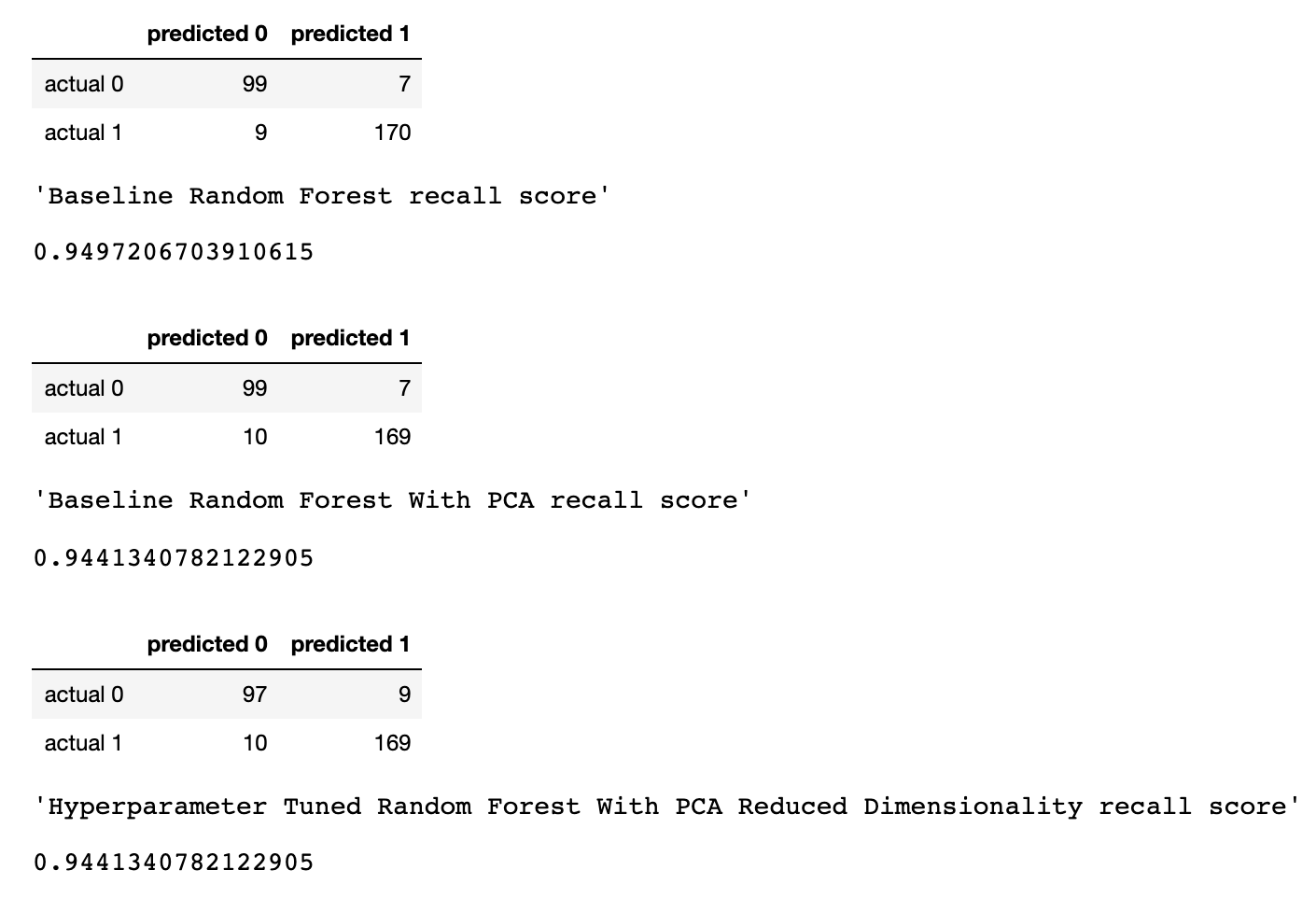
Результаты работы трёх моделей
Здесь оценивается метрика «полнота» (recall). Дело в том, что мы имеем дело с диагнозом рака. Поэтому нас чрезвычайно интересует минимизация ложноотрицательных прогнозов, выдаваемых моделями.
Учитывая это, можно сделать вывод о том, что базовая RF-модель дала наилучшие результаты. Её показатель полноты составил 94.97%. В проверочном наборе данных была запись о 179 пациентах, у которых есть рак. Модель нашла 170 из них.
Итоги
Это исследование позволяет сделать важное наблюдение. Иногда RF-модель, в которой используется метод главных компонент и широкомасштабная оптимизация гиперпараметров, может работать не так хорошо, как самая обыкновенная модель со стандартными настройками. Но это — не повод для того, чтобы ограничивать себя лишь простейшими моделями. Не попробовав разные модели, нельзя сказать о том, какая из них покажет наилучший результат. А в случае с моделями, которые используются для предсказания наличия у пациентов рака, можно сказать, что чем лучше модель — тем больше жизней может быть спасено.
Уважаемые читатели! Какие задачи вы решаете, привлекая методы машинного обучения?