Learning rate python что это
Learning Rate is an important hyperparameter in Gradient Descent. Its value determines how fast the Neural Network would converge to minima. Usually, we choose a learning rate and depending on the results change its value to get the optimal value for LR. If the learning rate is too low for the Neural Network the process of convergence would be very slow and if it’s too high the converging would be fast but there is a chance that the loss might overshoot. So we usually tune our parameters to find the best value for the learning rate. But is there a way we can improve this process?
Why adjust Learning Rate?
Instead of taking a constant learning rate, we can start with a higher value of LR and then keep decreasing its value periodically after certain iterations. This way we can initially have faster convergence whilst reducing the chances of overshooting the loss. In order to implement this we can use various scheduler in optim library in PyTorch. The format of a training loop is as following:-
Commonly used Schedulers in torch.optim.lr_scheduler
PyTorch provides several methods to adjust the learning rate based on the number of epochs. Let’s have a look at a few of them:–
- StepLR: Multiplies the learning rate with gamma every step_size epochs. For example, if lr = 0.1, gamma = 0.1 and step_size = 10 then after 10 epoch lr changes to lr*step_size in this case 0.01 and after another 10 epochs it becomes 0.001.
- MultiStepLR: This is a more customized version of StepLR in which the lr is changed after it reaches one of its epochs. Here we provide milestones that are epochs at which we want to update our learning rate.
- ExponentialLR: This is an aggressive version of StepLR in LR is changed after every epoch. You can think of it as StepLR with step_size = 1.
- ReduceLROnPlateau: Reduces learning rate when a metric has stopped improving. Models often benefit from reducing the learning rate by a factor of 2-10 once learning stagnates. This scheduler reads a metrics quantity and if no improvement is seen for a patience number of epochs, the learning rate is reduced.
Training Neural Networks using Schedulers
For this tutorial we are going to be using MNIST dataset, so we’ll start by loading our data and defining the model afterwards. Its recommended that you know how to create and train a Neural Network in PyTorch. Let’s start by loading our data.
Now that we have our dataloader ready we can now proceed to create our model. PyTorch model follows the following format:-
With that clear let’s define our model:-
Now that we have our model we can specify our optimizer, loss function and our lr_scheduler. We’ll be using SGD optimizer, CrossEntropyLoss for loss function and ReduceLROnPlateau for lr scheduler.
Let’s define the training loop. The training loop is pretty much the same as before except this time we’ll call our scheduler step method at the end of the loop.
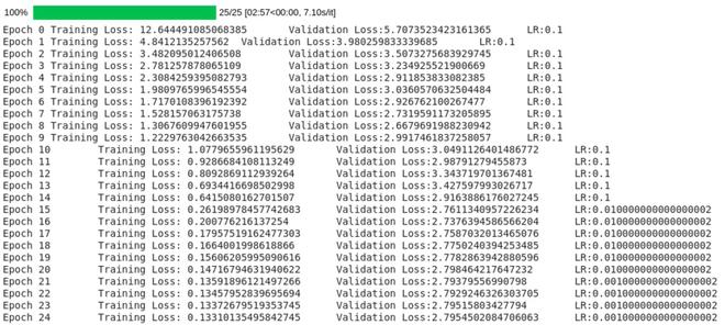
As you can see the scheduler kept adjusting lr when the validation loss stopped decreasing.
PyTorch: Learning Rate Schedules
Learning rate is one of the most important parameters of training a neural network that can impact the results of the network. When training a network using optimizers like SGD, the learning rate generally stays constant and does not change throughout the training process. Research has shown that as we train for more epochs, decreasing the learning rate little can improve the performance of the network. It can give a little boost to performance. The learning rate can be reduced after each epoch or batch. This process of decreasing the learning rate over time during the training process is generally referred to as learning rate scheduling or learning rate annealing in the machine learning community. Over time, there are various approaches tried to decrease the learning rate.
As a part of this tutorial, we’ll be discussing various learning rate schedules available from PyTorch. We have tried to cover the majority of schedules available from it. We have chosen the Fashion MNIST dataset for our tutorial and will be training a simple CNN on it. We’ll train CNN with various learning rate schedules and compare their results. We have also created visualizations showing how the learning rate changes during the training process. We are assuming that the reader has little background on Pytorch. Please feel free to check the below tutorial if you want to learn about CNN creation using Pytorch.
PyTorch let us change the learning rate in two different ways during the training process.
- After completion of each batch.
- After completion of each epoch.
We can modify code based on our requirements on when we want to change the learning rate. It even let us use more than one learning rate scheduler together which can be executed one after another to modify the learning rate using different formulas. We have explained in one of our examples how we can combine multiple learning rate schedulers as well.
Below, we have listed important sections of tutorial to give an overview of the material covered.
Important Sections of Tutorial
Below, we have imported PyTorch and printed the version that we have used in our tutorial.
Load Data 
In this section, we have loaded the Fashion MNIST dataset available from keras. The data has grayscale images of shape (28,28) pixels for 10 different fashion items. The dataset is already divided into the train (60k images) and test (10k images) sets. The below table has a mapping from index value to category name of the images.
| Label | Description |
|---|---|
| 0 | T-shirt/top |
| 1 | Trouser |
| 2 | Pullover |
| 3 | Dress |
| 4 | Coat |
| 5 | Sandal |
| 6 | Shirt |
| 7 | Sneaker |
| 8 | Bag |
| 9 | Ankle boot |
The keras provides dataset as numpy arrays whereas PyTorch networks require tensors hence we have converted them to PyTorch tensors. Later on, we have also created Dataset and DataLoader objects from tensors. The data loader objects will let us loop through data during the training process easier. We have kept a batch size of 128 samples when creating loader objects for train and test datasets.
Define CNN 
In this section, we have defined our convolutional neural network using Pytorch. Our network consists of 3 convolution layers and one linear layer. The convolution layers have 32, 16, and 8 output filters respectively. The kernel size of filters used by all three convolution layers is (3,3). We have also applied relu activation function to the output of each convolution layer. The output of the third convolution layer is flattened and then given as input to the linear layer. The linear layer has 10 units which are the same as the number of target classes.
1. Constant Learning Rate 
In this section, we are training our network with a constant learning rate. We’ll be recording the accuracy of the model on test data with various learning rate schedules along with a constant learning rate for comparison purposes later.
Below, we have designed three functions that we’ll use for training. There is one main training function that takes model, loss function, train loader, validation loader, and a number of epochs as input. It then executes the training loop number of epochs times. During each epoch, it performs a forward pass through the network to make predictions, calculate loss, calculate gradients, and update network parameters. It also records the loss of each batch and prints the average training loss after completion of each epoch. At the end of each epoch, it even calculates validation accuracy and validation loss using the other two helper functions defined in the below cell. The training function returns validation accuracy after completion of total training.
Below, we have initialized a dictionary named scheduler_val_accs that will hold the test accuracy of each learning rate schedule that we’ll try. We’ll also include constant learning rate results for comparison purposes.
In the next cell, we are actually training our network using the training function defined in the previous cell. We have initialized a number of epochs to 15 and the learning rate to 0.001. Followed by it, we have initialized our network, loss function, and optimizer. Then, we have called our training function with the necessary parameters to perform the training of the network. The function returns test accuracy which we have recorded in the dictionary. We are treating the test dataset as a validation dataset in our training process.
Using Learning Rate Scheduler and Early Stopping with PyTorch
In this tutorial, we will be focusing on two simple yet important concepts in regard to deep learning training. They are learning rate scheduler and early stopping. Further in the article, you will get to know how to use learning rate scheduler and early stopping with PyTorch while training your deep learning models.
Now, this concept may not be too advanced but are just as important for any newcomer to the field. So, if you are new to deep learning or starting out with deep learning with PyTorch, then I hope that this article helps.
So, what will we cover in this article?
- A brief about learning rate scheduler and early stopping in deep learning.
- Implementing learning rate scheduler and early stopping with PyTorch. We will use a simple image classification dataset for training a deep learning model.
- Then we will train our deep learning model:
- Without either early stopping or learning rate scheduler.
- With early stopping.
- With learning rate scheduler.
And each time observe how the loss and accuracy values vary. This will give us a pretty good idea of how early stopping and learning rate scheduler with PyTorch works and helps in training as well.
Note: We will not write any code to implement any advanced callbacks for early stopping and learning rate scheduler with PyTorch. We will use very simple code and that will give us an idea of how these work. This will also help new learners understand how to implement early stopping and learning rete scheduler with PyTorch code. Further on, they can integrate with any training code they want.
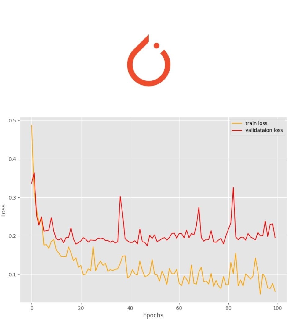
Figure 1. In this tutorial, you will get to learn to use learning rate scheduler and early stopping with PyTorch.
I hope that you are interested to follow this tutorial till the end. Let’s start with learning a bit about learning rate scheduler and early stopping in deep learning.
Learning Rate Scheduler
While training very large and deep neural networks, the model might overfit very easily. This becomes a larger issue when the dataset is small and simple. We can easily know this when while training, the validation loss, and training loss gradually start to diverge. This means that the model is starting to overfit. Also, using a single and high-value learning rate might cause the model to miss the local optima altogether during the last phases of training. During the last phases, the parameters should be updated gradually, unlike the initial training phases.
Trying to train a large neural network while using a single static learning rate is really difficult. This is where learning rate scheduler helps. Using learning rate scheduler, we can gradually decrease the learning rate value dynamically while training. There are many ways to do this. But the most commonly used method is when the validation loss does not improve for a few epochs.
Let’s say that we observe that the validation loss has not decreased for 5 consecutive epochs. Then there is a very high chance that the model is starting to overfit. In that case, we can start to decrease the learning rate, say, by a factor of 0.5.
We can continue to this for a certain number of epochs. When we are sure that the learning rate is so low that the model will not learn anything, then we can stop the training.
Early Stopping
Early stopping is another mechanism where we can prevent the neural network from overfitting on the data while training.
In early stopping, when we see that the training and validation loss plots are starting to diverge, then we just terminate the training. This is usually done in these two cases:
- We are very sure that the model is starting to overfit.
- We are also sure that using learning rate scheduler to reduce learning rate and more training will not help the model.
It actually depends on the machine learning engineer/researcher which to use of the two. While training large and deep learning neural networks on very large datasets, it is more common to use learning rate scheduler so that we are very sure that the neural network has reached the optimum solution.
We will not go into more theoretical details here. In the rest of the tutorial, we will see how to implement learning rate scheduler and early stopping with PyTorch.
Directory Structure and the Input Data
Now, let’s take a look at how to setup the directory for this mini-project.
- First, we have the input folder. Inside that, we have the alien-vs-predator-images and then data as the subfolders. The data folder contains the respective training and validation images for the alien class and the predator class.
- Then we have the outputs folder which will contain all the loss and accuracy plots along with the trained model after we have completed the training.
- Finally, we have the src folder which contains the four Python files in which we will be writing the code.
Coming to the data, we will be using Alien vs. Predator images from Kaggle. This is a very small dataset containing somewhere around 900 images belonging to the predator and alien classes. You can go ahead and download the dataset.
After downloading, extract it inside the input folder. The actual images that we will be using are inside the alien-vs-predator-images/data . So, if you see any other folders, you can ignore them as they are just a repetition of the images.

Figure 2. Some sample images from the Alien vs. Predator dataset that we will use in this tutorial.
Just to have an idea, figure 2 shows a few images from the dataset belonging to the alien and predator classes. This is a very basic image classification dataset. We will not focus much on it. Instead, we will focus on the important concept at hand, implementing learning rate scheduler and early stopping with Pytorch.
Libraries and Dependencies
As we will use the PyTorch deep learning framework, let’s clarify the version. I am using PyTorch 1.7.1 for this tutorial, which is the latest at the time of writing the tutorial.
There are other basic computer vision library dependencies as well, which most probably you already have. If you find missing anything, just install them as you go.
Code for Learning Rate Scheduler and Early Stopping with PyTorch
From this section onward, we will write the code for implementing learning rate scheduler and early stopping with PyTorch.
We have four 4 Python files and we will tackle them one at a time. So, let’s move onward and start writing the code.
Writing the Learning Rate Scheduler and Early Stopping Classes
To implement the learning rate scheduler and early stopping with PyTorch, we will write two simple classes.
The code that we will write in this section will go into the utils.py Python file. We will write the two classes in this file.
Starting with the learning rate scheduler class.
The Learning Rate Scheduler Class
Actually, PyTorch provides many learning rate schedulers already. And we will also be using one of that, ReduceLROnPlateau() to be particular. Then why write a class again for that? Well, we will try to write the code in such a way that using the functions will become easier and also it will adhere to the coding style of early stopping which we will implement later.
The following code block contains the complete learning rate scheduler class, that is LRScheduler() .
For, the whole utils.py file, we just need the torch module.
Coming to the LRScheduler class, I have provided the necessary documentation for easier understanding. This class will reduce the learning rate by a certain factor when the validation loss does not decrease for a certain number of epochs. Specifically, when the learning rate scheduler is executed internally, then the new_learning_rate = old_learning_rate * factor . So, smaller the factor , the lower the new learning rate value will be.
Going over the code briefly.
First, the __init__() function.
- This accepts the optimizer , patience , min_lr , and factor as parameters. You may read the description in the code documentation to know what each parameter does.
- The patience , min_lr , and factor have some initial values.
- From lines 20 to 23, we initialize the four variables first.
- At line 25, we initialize the self.lr_scheduler object of the ReduceLROnPlateau() class. Let’s go over the arguments it takes. First is the optimizer that we have provided. Then we have mode . It can be either min or max . We are using min which means that the learning rate will be updated when the metric that we are monitoring has stopped reducing. This is apt when we use validation loss as the monitoring metric. Then we have the patience , factor , and min_lr . min_lr defines the minimum value that the learning rate will reduce to. Finally, verbose=True will print a message whenever the learning rate is updated.
Secondly, the __call__() function.
This function contains just one line of code. That is, to take one step of the learning rate scheduler while providing the validation loss as the argument. The __call__() function will be executed whenever we will provide the validation loss as an argument to the object of the LRScheduler() class. Things will become clearer when we will actually use this in the training script.
Moving ahead, we will write the code for early stopping.
The Early Stopping Class
Now, Pytorch does not have any pre-defined class for early stopping. Therefore, we will write a very simple logic for that.
The following block contains the code for the early stopping class.
Going over all the variables in the __init__() function.
- self.patience defines the number of times we allow the validation loss to not improve before we early stop our training. Mind that this is not the number of consecutive epochs. Rather it is the cumulative number of times the validation loss does not improve during the whole training process.
- self.min_delta is the minimum difference between the new loss and the best loss for the new loss to be considered an improvement.
- Then we have self.counter which keeps count of the number of times the current validation loss does not improve.
- Finally, we have self.best_loss and self.early_stop which are None and False respectively.
Then we have the __call__() function which implements the early stopping logic. At the beginning of training, we make the current loss as the best loss at line 56. Line 57 checks whether the current loss is less than the best loss by the min_delta amount. If so, then we update the best validation loss value. If not, we increment the counter by 1 at line 60. Whenever the counter is greater than the patience value, then we update the self.early_stop to True and print some information on the screen. After this, further actions will be taken in the training script.
That’s it for the learning rate scheduler and early stopping code.
Preparing the Dataset
In this section, we will prepare the dataset that we will train our deep learning model on. Before moving further, make sure that you have downloaded the dataset and achieved the directory structure as discussed before.
We will write the code in dataset.py Python file for preparing the dataset.
For preparing the dataset, we will use the ImageFolder module of PyTorch. This will make our work way easier as we already have our extracted dataset in the way the ImageFolder module expects it to be.
Actually, by using the ImageFolder module, we can completely get rid of our custom dataset class and quickly move on to the training. It has its advantages and disadvantages, but for this tutorial, we want to focus on early stopping and learning rate scheduler.
The ImageFolder expects the dataset to be in the following format.
And our dataset is already in that format. Let’s take a look at our dataset folder structure a bit.
So, up till train and validation folders, it will be the root path and we can easily prepare the training and validation sets.
So, let’s get down to writing the code in dataset.py .
Starting off with the libraries and modules that we need.
Next, let’s define the image transforms and augmentations for training and validation.
For the training transforms, we are:
- Resizing all the images to 224×224 dimensions.
- Flipping the images horizontally and vertically with a random probability.
- Converting the images to tensors which divides all the pixel values by 255.0 and changes the dimension format to [channel, height, width].
- Normalizing all the pixel values by using the ImageNet normalization stats.
For the validation transforms, we do not apply any augmentations like flipping that we did in the case for training.
Finally, the training and validation datasets and dataloaders.
We are applying the respective transforms for training and validation datasets. The batch size for the data loaders is 32 and we are shuffling the training data loaders as well. Now, our data loaders are ready for training.
The Deep Learning Model
We will use an ImageNet pre-trained model in this tutorial. Specifically, we will use the ResNet50 pre-trained model.
We will freeze all the hidden layer parameters and make only the classification layer learnable.
The code here will go into the models.py Python file.
The following code block contains all the code we need for preparing the model.
At line 5, we are loading the ResNet50 model with the ImageNet pre-trained weights. As we will pass requires_grad=False , so, all the intermediate model parameters will be frozen. The final classification layer at line 14 has 2 output features. This corresponds to the two classes that we have, alien and predator. Finally, we return the model.
Moving ahead, we will start writing our training script.
Training Script for Learning Rate Scheduler and Early Stopping with PyTorch
This is the final code file that we will deal with in this tutorial. It is the training script that we will execute, the train.py Python file.
As always, the first code block contains all the libraries and modules that we will need for the training script.
At lines 10 and 11, we are importing the train_dataset , val_dataset and train_dataloader , and val_dataloader from dataset . We are also importing EarlyStopping and LRScheduler from utils at line 12.
Construct the Argument Parser and Initialize the Model
We will write the code to construct the argument parser which will tell whether we want to apply learning rate scheduler or early stopping.
So, while executing train.py , we can either provide —lr-scheduler or —early-stopping as the command line arguments. The code will be executed accordingly.
The next code block defines the computation device and loads the deep learning model as well.
Starting from line 26, we calculate the total number of parameters in the model. We also print the information on the screen about the total number of parameters and the number of trainable parameters.
The Learning Parameters
Now, we will define the learning/training parameters which include the learning rate, epochs, the optimizer, and the loss function.
We will be starting off with a learning rate of 0.001 and we will train for 100 epochs. The optimizer is the Adam optimizer and we are using the Cross Entropy loss function.
Initializing Learning Rate Scheduler and Early Stopping According to Command Line Arguments
While running the training script, we can either run it as it is, or we can provide either of the command line arguments for utilizing either the learning rate scheduler or early stopping. In that case, we can define some variable names for the loss plot, accuracy plot, and model so that they will be saved to disk with different names.
If we are neither using learning rate scheduler nor early stopping, then we will use the simple strings in the above code block. Else, we will initialize the learning rate scheduler and early stopping and change the variable names accoringly.
In the above code block, we are initializing the learning rate scheduler and early stopping according to the command line argument that is provided. Along with that, we also changing the plot and model names that we will use to save loss & accuracy plots and the trained model to disk.
The Training Function
The training function is going to be the standard PyTorch classification training function that we usually see. We will call the function fit() .
The first task is to put the model into training mode, which we are doing at line 62. We define train_running_loss and train_running_correct to keep track of the loss values and accuracy in each iteration. Starting from line 68, we iterate through the batches of data. We perform the standard operations like getting the batch loss, number of correct predictions, calculating the gradients, and updating the model parameters. After each epoch, we calculate the train_loss and train_accuracy and return those values (lines 81 to 83).
The Validation Function
The validation function will be very similar to the training function. Except, we need neither backpropagate the loss for gradient calculation nor update the model parameters.
Note that we are doing all the model predictions inside the with torch.no_grad() block. This ensures that we are not calculating any gradients which saves memory and time while validating. As in the case of training, we are returning the validation loss and accuracy at the end.
The Training Loop
As we have coded above, we will train and validate the model for 200 epochs. We can do that using a simple for loop. There are some other details that we need to take care of within the training loop. Let’s write the code, then we will get into those details.
First, at lines 109 and 110, we initialize four lists, train_loss , train_accuracy & val_loss , val_accuracy . They will store the training loss & accuracy and validation loss & accuracy for each epoch while training.
We start the training from line 112. At lines 114 and 117, we call the fit() and validate() functions by providing the required arguments. From lines 120 to 123, we append the accuracy and loss values to the respective lists.
The important stuff starts from line 124. If we provide —lr-scheduler command line argument while executing the training script, then the learning rate scheduler’s __call__() method will be executed at line 125. This in-turn makes the scheduler take one step by taking the current validation loss as the argument.
Else, if we provide —early-stopping command line argument while executing the training script, then lines 126 to 129 will be executed. Line 127 executes the __call__() method of the EarlyStopping() class. At line 128, we check whether the early_stop variable of the class is True . If so, then we print the early stopping message and break out of the training loop.
Finally, we just need to plot and save the accuracy and loss graphs. Along with that we will also save the trained model to disk. The following code block does that.
This marks the end of the training script as well as all the code that we need for this tutorial. We are all set to execute our training script.
Executing the train.py Script
Now it is time to execute our training script and analyze how everything is affected while using learning rate scheduler and early stopping with PyTorch.
First, we will train our model for 100 epochs without using learning rate scheduler or early stopping. Open up your terminal/command line in the src folder and type the following command.
You should see output similar to the following.
The final epoch gives a validation accuracy of 89% and validation loss of 0.1956. Let’s analyze the graphical plots saved on the disk and get some more information.
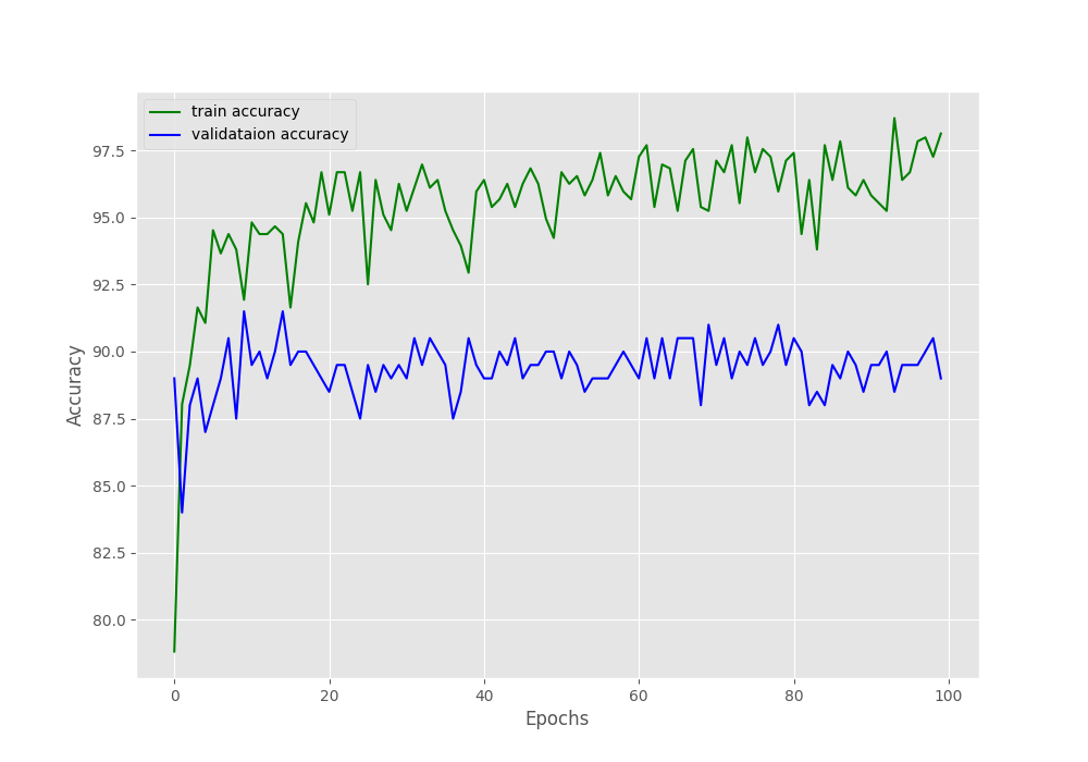
Figure 3. The accuracy plot after training for 100 epochs without learning rate scheduler or early stopping. We can see a lot of fluctuations in the plots.
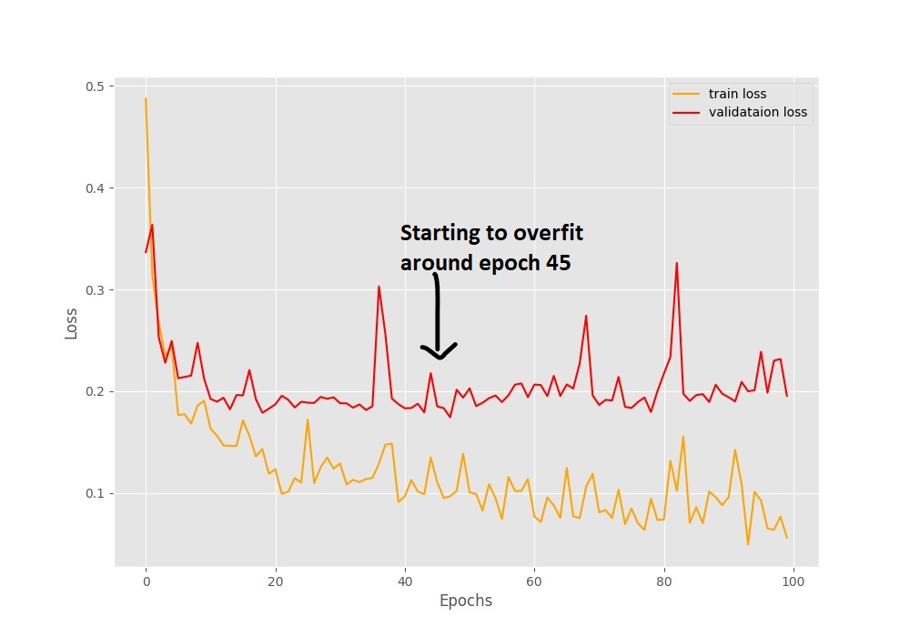
Figure 4. The loss plot after training for 100 epochs. The validation loss is starting to diverge around epoch 45 indicating that the learning rate is too high.
In the accuracy plot in figure 3, we can see a lot of fluctuations. The ups and downs are very severe between some of the epochs where the accuracy is differing by more than 3%. The loss plot also shows a similar trend but provides us with some more info. We can see that around epoch 45, the validation loss line starts to diverge (move upward). This is a clear indication that the model is starting to overfit and we need to reduce the learning rate for proper training to continue.
Now, let’s execute the training script along with learning rate scheduler and see whether this make a difference.
The following is the sample output.
If you observe the outputs on your console, then you will get to see all the instances where the learning rate scheduler kicks in.
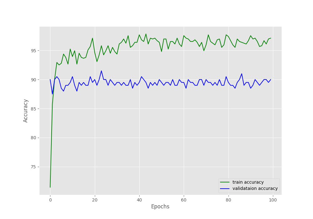
Figure 5. The accuracy plots when using learning rate scheduler are much smoother. Still, this indicates that the model might also overfit on the data.
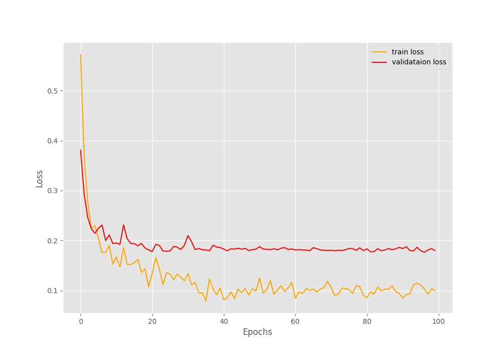
Figure 6. The validation loss plot does not diverge when in this case. This means that using learning rate scheduler we can control the learning rate effectively.
We can clearly see that the accuracy plot is a lot smoother here. By the end of the training, we are getting a validation accuracy of 90% which is higher than the previous case.
Figure 6 provides us with more useful information. This time, there is no divergence of the validation loss plot. This means that using learning rate scheduler actually worked. But if you observe closely, the validation loss starts to plateau around epoch 55. This means that we can train our model for 50-55 epochs and still get good results.
Finally, let’s use early stopping with our training script.
The training stopped after the validation loss did not improve 5 times in total. And our training stopped after 14 epochs. The following are the loss and accuracy plots. The final validation accuracy is comparable to the learning rate schedule case but the loss is obviously higher.
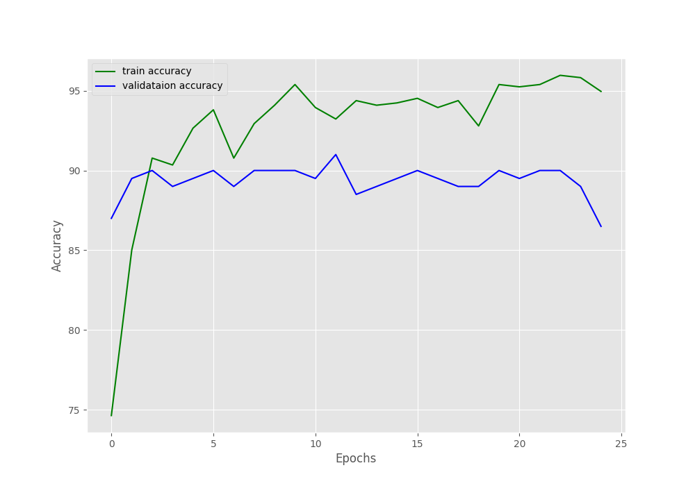
Figure 7. The accuracy plot when using early stopping. The training early stopped after 25 epochs.
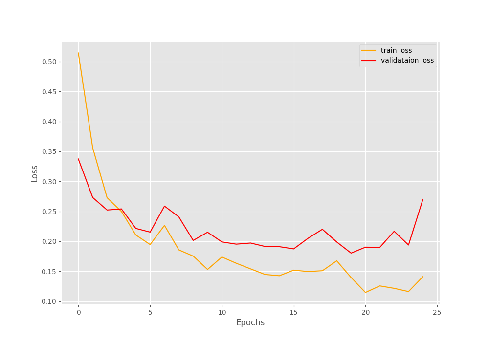
Figure 8. The loss plots when using early stopping. The training stopped when the validation loss did not improve for 5 epochs in total.
The accuracy and loss plots show the results for the 6 epochs only. Such an early end of training might result in the model not learning properly.
Although early stopping stopped the training after 6 epochs, it is very clear that using a learning rate scheduler and continuing training for more epochs is helpful. We inferred that from the previous case also. Maybe we do not need to train for 100 epochs, around 50-55 epochs is a good amount of training for the model to learn.
Summary and Conclusion
In this tutorial, you got to learn how to use the learning rate scheduler and early stopping with PyTorch. You also saw how both affect deep learning training and where they can be used to obtain better results. I hope that you learned something new.
If you have any doubts, thoughts, or suggestions, then please leave them in the comment section. I will surely address them.
You can contact me using the Contact section. You can also find me on LinkedIn, and Twitter.
14 thoughts on “Using Learning Rate Scheduler and Early Stopping with PyTorch”
Hi Sovit,
First of all, thanks for sharing.
I notice you set the default patience for both ‘lr_scheduler’ and ‘early_stopping’ as 5. So if run with the default patience, early_stopping will stop the training right after lr_scheduler reducing the learning rate. Wouldn’t you want to set early_stopping’s patience greater than lr_scheduler’s so it has a chance to see if the halving the learning rate could reduce the validation error? That is maybe why you training stopped early before the optimal. RegardsHi Jeo. Thanks for reaching out. If you take a look, then we are not using ‘lr_scheduler’ and ‘early_stopping’ both in a single training cycle. We are using either ‘lr_scheduler’ or ‘early_stopping’. But if you really think that the code uses both at the same time at some point, then please point line number. I will surely correct that out.
Comprehensive Guide To Learning Rate Algorithms (With Python Codes)

Learning rate is an important hyperparameter that controls how much we adjust the weights in the network according to the gradient. The question most commonly asked in the field of Machine learning is “how do we know what is the right value for learning rate?”
Unfortunately, there is no one size fits all answer to this question. But, I will put forth some of the methods you can use that can help you estimate what value should be used.
This article covers the types of Learning Rate (LR) algorithms, the behaviour of learning rates with SGD and implementation of techniques to find out suitable LR values.
Types of LR algorithms
The learning rate algorithms are broadly classified into two categories:
- Constant Learning rate algorithm – As the name suggests, these algorithms deal with learning rates that remain constant throughout the training process. Stochastic Gradient Descent falls under this category.
Here, η represents the learning rate. The smaller the value of η, the slower the training and adjustment of weights. But if the value is too high, the model converges too quickly and results in a suboptimal solution.
- Adaptive learning rate algorithm – Here, the optimizers help in changing the learning rate throughout the process of training. Adam, Adagrad, Adadelta, RMSProp are some examples of adaptive learning rate algorithms. For the purpose of this article, I will be using stochastic gradient descent to find the optimal learning rate.
Stochastic Gradient Descent and Learning rate
Stochastic Gradient Descent (SGD) is one of the most common optimizers used in machine learning. Let us see how SGD looks for a single sample. Take a look at the loss function below.
where x is the input sample, y is the label, and θ is the weight. We can define the partial derivative cost function for a batch size equal to N as:
In its most basic form, the SGD works by updating the value of . that moves the weights in the direction opposite to the gradient value of the loss.
Unfortunately, when it comes to deep learning models, the reality is different. The local minima in case of smaller models are relatively shallow and are easy to get past. But, because of millions of parameters involved in the deep models, the local minima tends to be wider and thus creates a problem called plateaus. This is also called saddle because of how it looks. When this situation occurs, our learning model is stuck in the saddle and struggles to get out.
One solution to this is fixing our learning rate large enough to escape the saddle. Let us now look at the methods that can be used.
- Reduce LR on Plateau: This is one of the ways of moving out of the saddle. Every time the loss begins to plateau, the learning rate decreases by a set fraction. When the loss function succumbs to higher learning rate and keeps moving around in the saddle, reducing the learning rate can help the loss find a smoother surface to escape this.
- LR Finder: In this method, the learning rate is selected by taking a random value for the weight, calculating the loss and getting a learning rate for that value. Next, a small step is taken and the learning rate is recalculated for the new weight and loss. This process is plotted in a graph and the optimal LR is selected.
- Cyclic Learning Rate: This method eliminates the need to experimentally find the best values and schedule for global learning rates. Instead of monotonically decreasing the learning rate, this method lets the learning rate cyclically vary between boundaries.
Let us implement Cyclic LR and LR finder for CIFAR 10 to understand the difference and see the improvement in the accuracy.
We will import the required libraries and load our data.
Our data has been loaded and saved in variables, let us normalize the data and convert them to categorical data.
For simplification purposes, let us split our data into batches and augment the data using Image Datagenerator.
Let us do the same for test data as well
Now, build a CNN model with batch normalization and regularization function (for faster convergence) and bear in mind to use SGD optimizer
Do not worry about the lr that is assigned above. You can assign any value here since we will be overriding it soon.
In order to make the model work better, I will use the cutout function.
Let us go ahead and implement the LR finder algorithm from Keras.
It is time to put everything together. We will define our accuracy function and a function to plot the model graphically.
Typically, a good static learning rate can be found half-way on the descending loss curve. In the plot shown that would be around 0.002(10^-3) because that is where the descent is steeper.
For our cyclic learning rates, we need boundaries (start and end) and this can be identified from the graph as well. The boundaries are the point at which the loss starts descending and the point at which the loss stops descending. From the graph above, the curve starts at 0.002 and stops at 0.2 (10^-1). We have identified our boundaries, let us implement the cyclic LR and begin our training.
Although we see no sharp spikes, while tuning hyperparameters it is essential to check for overfitting. The best way to do this is to identify misclassified images in the dataset. Once this identification is done, you can always go back to the learning rate curves or the model and tweak it further to get the best results possible. I will use gradcam and identify the misclassifications below.
You can see here that these images are not classified right. But now that we have the tools to improve our learning rates we can go back to the model and tune it better.
Conclusion
Hyper-parameter optimization is a very important and time-consuming process in the life of a good machine learning model. It helps in making the model stand out and be better. With the techniques discussed above, you can improve your model by tuning the learning rates better.