Как закодировать категориальные признаки python

Guide to Encoding Categorical Values in Python

In many practical Data Science activities, the data set will contain categorical variables. These variables are typically stored as text values which represent various traits. Some examples include color (“Red”, “Yellow”, “Blue”), size (“Small”, “Medium”, “Large”) or geographic designations (State or Country). Regardless of what the value is used for, the challenge is determining how to use this data in the analysis. Many machine learning algorithms can support categorical values without further manipulation but there are many more algorithms that do not. Therefore, the analyst is faced with the challenge of figuring out how to turn these text attributes into numerical values for further processing.

As with many other aspects of the Data Science world, there is no single answer on how to approach this problem. Each approach has trade-offs and has potential impact on the outcome of the analysis. Fortunately, the python tools of pandas and scikit-learn provide several approaches that can be applied to transform the categorical data into suitable numeric values. This article will be a survey of some of the various common (and a few more complex) approaches in the hope that it will help others apply these techniques to their real world problems.

The Data Set

For this article, I was able to find a good dataset at the UCI Machine Learning Repository. This particular Automobile Data Set includes a good mix of categorical values as well as continuous values and serves as a useful example that is relatively easy to understand. Since domain understanding is an important aspect when deciding how to encode various categorical values — this data set makes a good case study.

Before we get started encoding the various values, we need to important the data and do some minor cleanups. Fortunately, pandas makes this straightforward:

symboling	normalized_losses	make	fuel_type	aspiration	num_doors	body_style	drive_wheels	engine_location	wheel_base	…	engine_size	fuel_system	bore	stroke	compression_ratio	horsepower	peak_rpm	city_mpg	highway_mpg	price
0	3	NaN	alfa-romero	gas	std	two	convertible	rwd	front	88.6	…	130	mpfi	3.47	2.68	9.0	111.0	5000.0	21	27	13495.0
1	3	NaN	alfa-romero	gas	std	two	convertible	rwd	front	88.6	…	130	mpfi	3.47	2.68	9.0	111.0	5000.0	21	27	16500.0
2	1	NaN	alfa-romero	gas	std	two	hatchback	rwd	front	94.5	…	152	mpfi	2.68	3.47	9.0	154.0	5000.0	19	26	16500.0
3	2	164.0	audi	gas	std	four	sedan	fwd	front	99.8	…	109	mpfi	3.19	3.40	10.0	102.0	5500.0	24	30	13950.0
4	2	164.0	audi	gas	std	four	sedan	4wd	front	99.4	…	136	mpfi	3.19	3.40	8.0	115.0	5500.0	18	22	17450.0

The final check we want to do is see what data types we have:

Since this article will only focus on encoding the categorical variables, we are going to include only the object columns in our dataframe. Pandas has a helpful select_dtypes function which we can use to build a new dataframe containing only the object columns.

make	fuel_type	aspiration	num_doors	body_style	drive_wheels	engine_location	engine_type	num_cylinders	fuel_system
0	alfa-romero	gas	std	two	convertible	rwd	front	dohc	four	mpfi
1	alfa-romero	gas	std	two	convertible	rwd	front	dohc	four	mpfi
2	alfa-romero	gas	std	two	hatchback	rwd	front	ohcv	six	mpfi
3	audi	gas	std	four	sedan	fwd	front	ohc	four	mpfi
4	audi	gas	std	four	sedan	4wd	front	ohc	five	mpfi

Before going any further, there are a couple of null values in the data that we need to clean up.

make	fuel_type	aspiration	num_doors	body_style	drive_wheels	engine_location	engine_type	num_cylinders	fuel_system
27	dodge	gas	turbo	NaN	sedan	fwd	front	ohc	four	mpfi
63	mazda	diesel	std	NaN	sedan	fwd	front	ohc	four	idi

For the sake of simplicity, just fill in the value with the number 4 (since that is the most common value):

Now that the data does not have any null values, we can look at options for encoding the categorical values.

Approach #1 — Find and Replace

Before we go into some of the more “standard” approaches for encoding categorical data, this data set highlights one potential approach I’m calling “find and replace.”

There are two columns of data where the values are words used to represent numbers. Specifically the number of cylinders in the engine and number of doors on the car. Pandas makes it easy for us to directly replace the text values with their numeric equivalent by using replace .

We have already seen that the num_doors data only includes 2 or 4 doors. The number of cylinders only includes 7 values and they are easily translated to valid numbers:

If you review the replace documentation, you can see that it is a powerful command that has many options. For our uses, we are going to create a mapping dictionary that contains each column to process as well as a dictionary of the values to translate.

Here is the complete dictionary for cleaning up the num_doors and num_cylinders columns:

To convert the columns to numbers using replace :

make	fuel_type	aspiration	num_doors	body_style	drive_wheels	engine_location	engine_type	num_cylinders	fuel_system
0	alfa-romero	gas	std	2	convertible	rwd	front	dohc	4	mpfi
1	alfa-romero	gas	std	2	convertible	rwd	front	dohc	4	mpfi
2	alfa-romero	gas	std	2	hatchback	rwd	front	ohcv	6	mpfi
3	audi	gas	std	4	sedan	fwd	front	ohc	4	mpfi
4	audi	gas	std	4	sedan	4wd	front	ohc	5	mpfi

The nice benefit to this approach is that pandas “knows” the types of values in the columns so the object is now a int64

While this approach may only work in certain scenarios it is a very useful demonstration of how to convert text values to numeric when there is an “easy” human interpretation of the data. This concept is also useful for more general data cleanup.

Approach #2 — Label Encoding

Another approach to encoding categorical values is to use a technique called label encoding. Label encoding is simply converting each value in a column to a number. For example, the body_style column contains 5 different values. We could choose to encode it like this:

• convertible -> 0
• hardtop -> 1
• hatchback -> 2
• sedan -> 3
• wagon -> 4

This process reminds me of Ralphie using his secret decoder ring in “A Christmas Story”

One trick you can use in pandas is to convert a column to a category, then use those category values for your label encoding:

Then you can assign the encoded variable to a new column using the cat.codes accessor:

make	fuel_type	aspiration	num_doors	body_style	drive_wheels	engine_location	engine_type	num_cylinders	fuel_system	body_style_cat
0	alfa-romero	gas	std	2	convertible	rwd	front	dohc	4	mpfi	0
1	alfa-romero	gas	std	2	convertible	rwd	front	dohc	4	mpfi	0
2	alfa-romero	gas	std	2	hatchback	rwd	front	ohcv	6	mpfi	2
3	audi	gas	std	4	sedan	fwd	front	ohc	4	mpfi	3
4	audi	gas	std	4	sedan	4wd	front	ohc	5	mpfi	3

The nice aspect of this approach is that you get the benefits of pandas categories (compact data size, ability to order, plotting support) but can easily be converted to numeric values for further analysis.

Approach #3 — One Hot Encoding

Label encoding has the advantage that it is straightforward but it has the disadvantage that the numeric values can be “misinterpreted” by the algorithms. For example, the value of 0 is obviously less than the value of 4 but does that really correspond to the data set in real life? Does a wagon have “4X” more weight in our calculation than the convertible? In this example, I don’t think so.

A common alternative approach is called one hot encoding (but also goes by several different names shown below). Despite the different names, the basic strategy is to convert each category value into a new column and assigns a 1 or 0 (True/False) value to the column. This has the benefit of not weighting a value improperly but does have the downside of adding more columns to the data set.

Pandas supports this feature using get_dummies. This function is named this way because it creates dummy/indicator variables (aka 1 or 0).

Hopefully a simple example will make this more clear. We can look at the column drive_wheels where we have values of 4wd , fwd or rwd . By using get_dummies we can convert this to three columns with a 1 or 0 corresponding to the correct value:

make	fuel_type	aspiration	num_doors	body_style	engine_location	engine_type	num_cylinders	fuel_system	body_style_cat	drive_wheels_4wd	drive_wheels_fwd	drive_wheels_rwd
0	alfa-romero	gas	std	2	convertible	front	dohc	4	mpfi	0	0.0	0.0	1.0
1	alfa-romero	gas	std	2	convertible	front	dohc	4	mpfi	0	0.0	0.0	1.0
2	alfa-romero	gas	std	2	hatchback	front	ohcv	6	mpfi	2	0.0	0.0	1.0
3	audi	gas	std	4	sedan	front	ohc	4	mpfi	3	0.0	1.0	0.0
4	audi	gas	std	4	sedan	front	ohc	5	mpfi	3	1.0	0.0	0.0

The new data set contains three new columns:

• drive_wheels_4wd
• drive_wheels_rwd
• drive_wheels_fwd

This function is powerful because you can pass as many category columns as you would like and choose how to label the columns using prefix . Proper naming will make the rest of the analysis just a little bit easier.

make	fuel_type	aspiration	num_doors	engine_location	engine_type	num_cylinders	fuel_system	body_style_cat	body_convertible	body_hardtop	body_hatchback	body_sedan	body_wagon	drive_4wd	drive_fwd	drive_rwd
0	alfa-romero	gas	std	2	front	dohc	4	mpfi	0	1.0	0.0	0.0	0.0	0.0	0.0	0.0	1.0
1	alfa-romero	gas	std	2	front	dohc	4	mpfi	0	1.0	0.0	0.0	0.0	0.0	0.0	0.0	1.0
2	alfa-romero	gas	std	2	front	ohcv	6	mpfi	2	0.0	0.0	1.0	0.0	0.0	0.0	0.0	1.0
3	audi	gas	std	4	front	ohc	4	mpfi	3	0.0	0.0	0.0	1.0	0.0	0.0	1.0	0.0
4	audi	gas	std	4	front	ohc	5	mpfi	3	0.0	0.0	0.0	1.0	0.0	1.0	0.0	0.0

The other concept to keep in mind is that get_dummies returns the full dataframe so you will need to filter out the objects using select_dtypes when you are ready to do the final analysis.

One hot encoding, is very useful but it can cause the number of columns to expand greatly if you have very many unique values in a column. For the number of values in this example, it is not a problem. However you can see how this gets really challenging to manage when you have many more options.

Approach #4 — Custom Binary Encoding

Depending on the data set, you may be able to use some combination of label encoding and one hot encoding to create a binary column that meets your needs for further analysis.

In this particular data set, there is a column called engine_type that contains several different values:

For the sake of discussion, maybe all we care about is whether or not the engine is an Overhead Cam ( OHC ) or not. In other words, the various versions of OHC are all the same for this analysis. If this is the case, then we could use the str accessor plus np.where to create a new column the indicates whether or not the car has an OHC engine.

I find that this is a handy function I use quite a bit but sometimes forget the syntax so here is a graphic showing what we are doing:

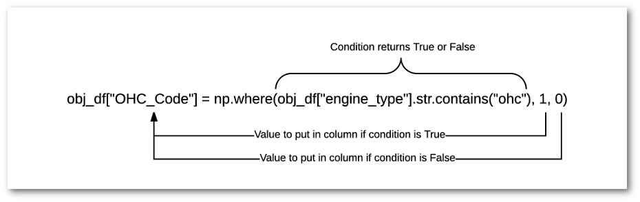
The resulting dataframe looks like this (only showing a subset of columns):

make	engine_type	OHC_Code
0	alfa-romero	dohc	1
1	alfa-romero	dohc	1
2	alfa-romero	ohcv	1
3	audi	ohc	1
4	audi	ohc	1

This approach can be really useful if there is an option to consolidate to a simple Y/N value in a column. This also highlights how important domain knowledge is to solving the problem in the most efficient manner possible.

Scikit-Learn

The previous version of this article used LabelEncoder and LabelBinarizer which are not the recommended approach for encoding categorical values. These encoders should only be used to encode the target values not the feature values.

The examples below use OrdinalEncoder and OneHotEncoder which is the correct approach to use for encoding target values.

In addition to the pandas approach, scikit-learn provides similar functionality. Personally, I find using pandas a little simpler to understand but the scikit approach is optimal when you are trying to build a predictive model.

For instance, if we want to do the equivalent to label encoding on the make of the car, we need to instantiate a OrdinalEncoder object and fit_transform the data:

make	make_code
0	alfa-romero	0
1	alfa-romero	0
2	alfa-romero	0
3	audi	1
4	audi	1
5	audi	1
6	audi	1
7	audi	1
8	audi	1
9	audi	1
10	bmw	2

Scikit-learn also supports binary encoding by using the OneHotEncoder. We use a similar process as above to transform the data but the process of creating a pandas DataFrame adds a couple of extra steps.

convertible	hardtop	hatchback	sedan	wagon
0	1	0	0	0	0
1	1	0	0	0	0
2	0	0	1	0	0
3	0	0	0	1	0
4	0	0	0	1	0

The next step would be to join this data back to the original dataframe. Here is an example:

The key point is that you need to use toarray() to convert the results to a format that can be converted into a DataFrame.

Advanced Approaches

There are even more advanced algorithms for categorical encoding. I do not have a lot of personal experience with them but for the sake of rounding out this guide, I wanted to included them. This article provides some additional technical background. The other nice aspect is that the author of the article has created a scikit-learn contrib package called category_encoders which implements many of these approaches. It is a very nice tool for approaching this problem from a different perspective.

Here is a brief introduction to using the library for some other types of encoding. For the first example, we will try doing a Backward Difference encoding.

First we get a clean dataframe and setup the BackwardDifferenceEncoder :

engine_type_0	engine_type_1	engine_type_2	engine_type_3	engine_type_4	engine_type_5
0	-0.857143	-0.714286	-0.571429	-0.428571	-0.285714	-0.142857
1	-0.857143	-0.714286	-0.571429	-0.428571	-0.285714	-0.142857
2	0.142857	-0.714286	-0.571429	-0.428571	-0.285714	-0.142857
3	0.142857	0.285714	-0.571429	-0.428571	-0.285714	-0.142857
4	0.142857	0.285714	-0.571429	-0.428571	-0.285714	-0.142857

The interesting thing is that you can see that the result are not the standard 1’s and 0’s we saw in the earlier encoding examples.

If we try a polynomial encoding, we get a different distribution of values used to encode the columns:

engine_type_0	engine_type_1	engine_type_2	engine_type_3	engine_type_4	engine_type_5
0	-0.566947	0.545545	-0.408248	0.241747	-0.109109	0.032898
1	-0.566947	0.545545	-0.408248	0.241747	-0.109109	0.032898
2	-0.377964	0.000000	0.408248	-0.564076	0.436436	-0.197386
3	-0.188982	-0.327327	0.408248	0.080582	-0.545545	0.493464
4	-0.188982	-0.327327	0.408248	0.080582	-0.545545	0.493464

There are several different algorithms included in this package and the best way to learn is to try them out and see if it helps you with the accuracy of your analysis. The code shown above should give you guidance on how to plug in the other approaches and see what kind of results you get.

scikit-learn pipelines

As mentioned above, scikit-learn’s categorical encoders allow you to incorporate the transformation into your pipelines which can simplify the model building process and avoid some pitfalls. I recommend this Data School video as a good intro. It also serves as the basis for the approach outlined below.

Here is a very quick example of how to incorporate the OneHotEncoder and OrdinalEncoder into a pipeline and use cross_val_score to analyze the results:

Now that we have our data, let’s build the column transformer:

This example shows how to apply different encoder types for certain columns. Using the remainder=’passthrough’ argument to pass all the numeric values through the pipeline without any changes.

For the model, we use a simple linear regression and then make the pipeline:

Run the cross validation 10 times using the negative mean absolute error as our scoring function. Finally, take the average of the 10 values to see the magnitude of the error:

Which yields a value of -2937.17.

There is obviously much more analysis that can be done here but this is meant to illustrate how to use the scikit-learn functions in a more realistic analysis pipeline.

Conclusion

Encoding categorical variables is an important step in the data science process. Because there are multiple approaches to encoding variables, it is important to understand the various options and how to implement them on your own data sets. The python data science ecosystem has many helpful approaches to handling these problems. I encourage you to keep these ideas in mind the next time you find yourself analyzing categorical variables. For more details on the code in this article, feel free to review the notebook.

sklearn.preprocessing .OrdinalEncoder¶

The input to this transformer should be an array-like of integers or strings, denoting the values taken on by categorical (discrete) features. The features are converted to ordinal integers. This results in a single column of integers (0 to n_categories — 1) per feature.

Read more in the User Guide .

New in version 0.20.

Categories (unique values) per feature:

‘auto’ : Determine categories automatically from the training data.

list : categories[i] holds the categories expected in the ith column. The passed categories should not mix strings and numeric values, and should be sorted in case of numeric values.

The used categories can be found in the categories_ attribute.

dtype number type, default np.float64

Desired dtype of output.

handle_unknown <‘error’, ‘use_encoded_value’>, default=’error’

When set to ‘error’ an error will be raised in case an unknown categorical feature is present during transform. When set to ‘use_encoded_value’, the encoded value of unknown categories will be set to the value given for the parameter unknown_value . In inverse_transform , an unknown category will be denoted as None.

New in version 0.24.

When the parameter handle_unknown is set to ‘use_encoded_value’, this parameter is required and will set the encoded value of unknown categories. It has to be distinct from the values used to encode any of the categories in fit . If set to np.nan, the dtype parameter must be a float dtype.

New in version 0.24.

Encoded value of missing categories. If set to np.nan , then the dtype parameter must be a float dtype.

New in version 1.1.

The categories of each feature determined during fit (in order of the features in X and corresponding with the output of transform ). This does not include categories that weren’t seen during fit .

n_features_in_ int

Number of features seen during fit .

New in version 1.0.

Names of features seen during fit . Defined only when X has feature names that are all strings.

New in version 1.0.

Performs a one-hot encoding of categorical features.

Encodes target labels with values between 0 and n_classes-1 .

With a high proportion of nan values, inferring categories becomes slow with Python versions before 3.10. The handling of nan values was improved from Python 3.10 onwards, (c.f. bpo-43475).

Given a dataset with two features, we let the encoder find the unique values per feature and transform the data to an ordinal encoding.

By default, OrdinalEncoder is lenient towards missing values by propagating them.

You can use the parameter encoded_missing_value to encode missing values.

Fit the OrdinalEncoder to X.

Fit to data, then transform it.

Get output feature names for transformation.

Get parameters for this estimator.

Convert the data back to the original representation.

Set output container.

Set the parameters of this estimator.

Transform X to ordinal codes.

Fit the OrdinalEncoder to X.

Parameters : X array-like of shape (n_samples, n_features)

The data to determine the categories of each feature.

y None

Ignored. This parameter exists only for compatibility with Pipeline .

Returns : self object

Fit to data, then transform it.

Fits transformer to X and y with optional parameters fit_params and returns a transformed version of X .

Parameters : X array-like of shape (n_samples, n_features)

y array-like of shape (n_samples,) or (n_samples, n_outputs), default=None

Target values (None for unsupervised transformations).

**fit_params dict

Additional fit parameters.

Returns : X_new ndarray array of shape (n_samples, n_features_new)

get_feature_names_out ( input_features = None ) [source] ¶

Get output feature names for transformation.

Parameters : input_features array-like of str or None, default=None

If input_features is None , then feature_names_in_ is used as feature names in. If feature_names_in_ is not defined, then the following input feature names are generated: ["x0", "x1", . "x(n_features_in_ — 1)"] .

If input_features is an array-like, then input_features must match feature_names_in_ if feature_names_in_ is defined.

Same as input features.

Get parameters for this estimator.

Parameters : deep bool, default=True

If True, will return the parameters for this estimator and contained subobjects that are estimators.

Returns : params dict

Parameter names mapped to their values.

Convert the data back to the original representation.

Parameters : X array-like of shape (n_samples, n_encoded_features)

The transformed data.

Returns : X_tr ndarray of shape (n_samples, n_features)

Inverse transformed array.

Set output container.

See Introducing the set_output API for an example on how to use the API.

Parameters : transform <“default”, “pandas”>, default=None

Configure output of transform and fit_transform .

"default" : Default output format of a transformer

"pandas" : DataFrame output

None : Transform configuration is unchanged

Set the parameters of this estimator.

The method works on simple estimators as well as on nested objects (such as Pipeline ). The latter have parameters of the form <component>__<parameter> so that it’s possible to update each component of a nested object.

Parameters : **params dict

Returns : self estimator instance

Transform X to ordinal codes.

Parameters : X array-like of shape (n_samples, n_features)

The data to encode.

Returns : X_out ndarray of shape (n_samples, n_features)

Name already in use

Work fast with our official CLI. Learn more about the CLI.

Sign In Required

Please sign in to use Codespaces.

Launching GitHub Desktop

If nothing happens, download GitHub Desktop and try again.

Launching GitHub Desktop

If nothing happens, download GitHub Desktop and try again.

Launching Xcode

If nothing happens, download Xcode and try again.

Launching Visual Studio Code

Your codespace will open once ready.

There was a problem preparing your codespace, please try again.

Latest commit

Git stats

Files

Failed to load latest commit information.

README.md

Categorical Encoding Methods

A set of scikit-learn-style transformers for encoding categorical variables into numeric by means of different techniques.

Unsupervised:

• Backward Difference Contrast [2][3]
• BaseN [6]
• Binary [5]
• Gray [14]
• Count [10]
• Hashing [1]
• Helmert Contrast [2][3]
• Ordinal [2][3]
• One-Hot [2][3]
• Rank Hot [15]
• Polynomial Contrast [2][3]
• Sum Contrast [2][3]

Supervised:

• CatBoost [11]
• Generalized Linear Mixed Model [12]
• James-Stein Estimator [9]
• LeaveOneOut [4]
• M-estimator [7]
• Target Encoding [7]
• Weight of Evidence [8]
• Quantile Encoder [13]
• Summary Encoder [13]

The package requires: numpy , statsmodels , and scipy .

To install the package, execute:

To install the development version, you may use:

All of the encoders are fully compatible sklearn transformers, so they can be used in pipelines or in your existing scripts. Supported input formats include numpy arrays and pandas dataframes. If the cols parameter isn’t passed, all columns with object or pandas categorical data type will be encoded. Please see the docs for transformer-specific configuration options.

There are two types of encoders: unsupervised and supervised. An unsupervised example:

And a supervised example:

For the transformation of the training data with the supervised methods, you should use fit_transform() method instead of fit().transform() , because these two methods do not have to generate the same result. The difference can be observed with LeaveOneOut encoder, which performs a nested cross-validation for the training data in fit_transform() method (to decrease over-fitting of the downstream model) but uses all the training data for scoring with transform() method (to get as accurate estimates as possible).

Furthermore, you may benefit from following wrappers:

• PolynomialWrapper, which extends supervised encoders to support polynomial targets
• NestedCVWrapper, which helps to prevent overfitting

Additional examples and benchmarks can be found in the examples directory.

Способы кодирования категориальных данных

В сфере data science подготовка данных является обязательным этапом работы перед построением моделей. Один из них — кодирование категориальных данных, т.к. значимая часть информации в реальной жизни относится именно к категориальным строковым значениям, а подавляющее большинство моделей умеют работать исключительно с числовыми значениями. Кодирование — это и есть процесс преобразования категориальных данных в числовой формат.

Содержание

Что такое категориальные данные?

Раз уж вся эта статья про категориальные данные, то давайте подробнее обсудим, что это такое. Если совсем кратно, то это данные с ограниченным числом уникальных значений или категорий.

Также к категориальным данным можно относиться как к значениям, которые делят все имеющиеся объекты изучения на группы. Например, список людей с их группой крови: I, II, III, IV. В таком списке каждая группа крови является категориальным значением.

Категориальные данные могут быть двух видов: порядковыми и номинальными.

Номинальные категории. Такие значения не могут быть проранжированы, и нет логической возможности их порядкового сравнения между собой. Например, это могут быть названия различных отделов в компании: производственный отдел, отдел кадров, бухгалтерия и так далее.

Выше представлено несколько примеров номинальных данных.

Порядковые категории. Такие значения могут быть упорядочены, и их можно сравниваться друг с другом. Например, показатель уровня сахара у пациентов, который можно представить как высокий, низкий и средний.

Выше представлены несколько примеров порядковых данных.

Label Encoding и Ordinal Encoding

Эти способы кодирования используется, когда категории являются порядковыми. Каждое уникальное значение преобразуется в целочисленное, таким образом, все значения просто преобразовываются в числовой ряд по возрастанию.