Как строить графики в python seaborn

An introduction to seaborn#

Seaborn is a library for making statistical graphics in Python. It builds on top of matplotlib and integrates closely with pandas data structures.

Seaborn helps you explore and understand your data. Its plotting functions operate on dataframes and arrays containing whole datasets and internally perform the necessary semantic mapping and statistical aggregation to produce informative plots. Its dataset-oriented, declarative API lets you focus on what the different elements of your plots mean, rather than on the details of how to draw them.

Here’s an example of what seaborn can do:

A few things have happened here. Let’s go through them one by one:

Seaborn is the only library we need to import for this simple example. By convention, it is imported with the shorthand sns .

Behind the scenes, seaborn uses matplotlib to draw its plots. For interactive work, it’s recommended to use a Jupyter/IPython interface in matplotlib mode, or else you’ll have to call matplotlib.pyplot.show() when you want to see the plot.

This uses the matplotlib rcParam system and will affect how all matplotlib plots look, even if you don’t make them with seaborn. Beyond the default theme, there are several other options , and you can independently control the style and scaling of the plot to quickly translate your work between presentation contexts (e.g., making a version of your figure that will have readable fonts when projected during a talk). If you like the matplotlib defaults or prefer a different theme, you can skip this step and still use the seaborn plotting functions.

Most code in the docs will use the load_dataset() function to get quick access to an example dataset. There’s nothing special about these datasets: they are just pandas dataframes, and we could have loaded them with pandas.read_csv() or built them by hand. Most of the examples in the documentation will specify data using pandas dataframes, but seaborn is very flexible about the data structures that it accepts.

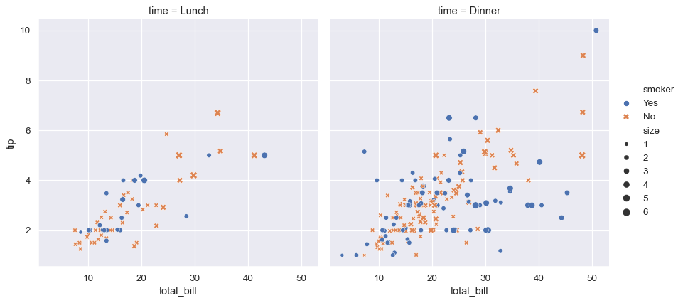
This plot shows the relationship between five variables in the tips dataset using a single call to the seaborn function relplot() . Notice how we provided only the names of the variables and their roles in the plot. Unlike when using matplotlib directly, it wasn’t necessary to specify attributes of the plot elements in terms of the color values or marker codes. Behind the scenes, seaborn handled the translation from values in the dataframe to arguments that matplotlib understands. This declarative approach lets you stay focused on the questions that you want to answer, rather than on the details of how to control matplotlib.

A high-level API for statistical graphics#

There is no universally best way to visualize data. Different questions are best answered by different plots. Seaborn makes it easy to switch between different visual representations by using a consistent dataset-oriented API.

The function relplot() is named that way because it is designed to visualize many different statistical relationships. While scatter plots are often effective, relationships where one variable represents a measure of time are better represented by a line. The relplot() function has a convenient kind parameter that lets you easily switch to this alternate representation:

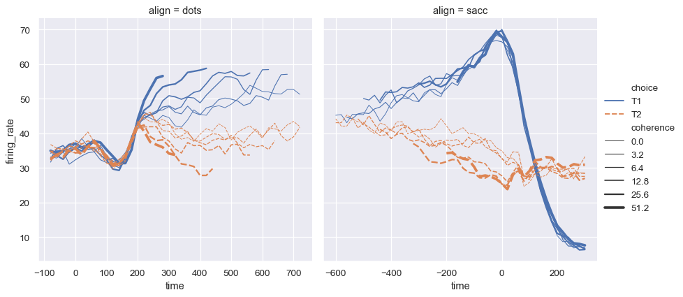
Notice how the size and style parameters are used in both the scatter and line plots, but they affect the two visualizations differently: changing the marker area and symbol in the scatter plot vs the line width and dashing in the line plot. We did not need to keep those details in mind, letting us focus on the overall structure of the plot and the information we want it to convey.

Statistical estimation#

Often, we are interested in the average value of one variable as a function of other variables. Many seaborn functions will automatically perform the statistical estimation that is necessary to answer these questions:

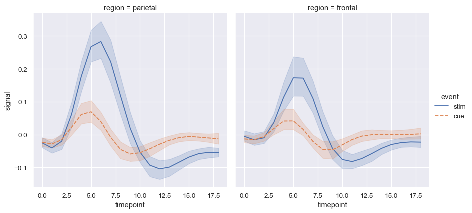
When statistical values are estimated, seaborn will use bootstrapping to compute confidence intervals and draw error bars representing the uncertainty of the estimate.

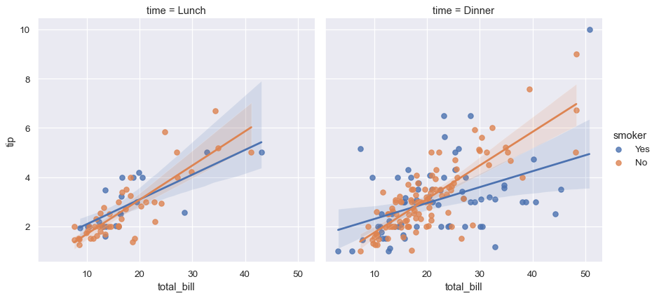
Statistical estimation in seaborn goes beyond descriptive statistics. For example, it is possible to enhance a scatterplot by including a linear regression model (and its uncertainty) using lmplot() :

Distributional representations#

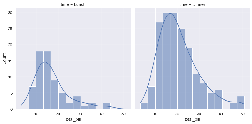
Statistical analyses require knowledge about the distribution of variables in your dataset. The seaborn function displot() supports several approaches to visualizing distributions. These include classic techniques like histograms and computationally-intensive approaches like kernel density estimation:

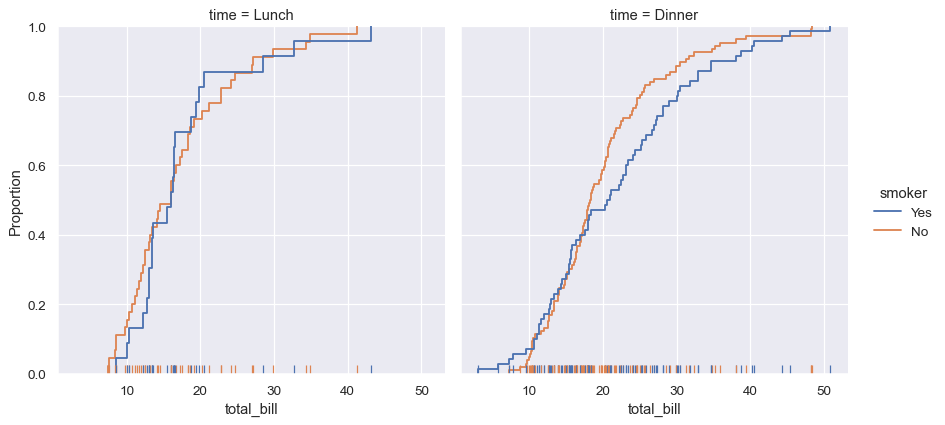
Seaborn also tries to promote techniques that are powerful but less familiar, such as calculating and plotting the empirical cumulative distribution function of the data:

Plots for categorical data#

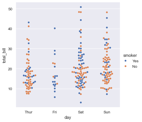
Several specialized plot types in seaborn are oriented towards visualizing categorical data. They can be accessed through catplot() . These plots offer different levels of granularity. At the finest level, you may wish to see every observation by drawing a “swarm” plot: a scatter plot that adjusts the positions of the points along the categorical axis so that they don’t overlap:

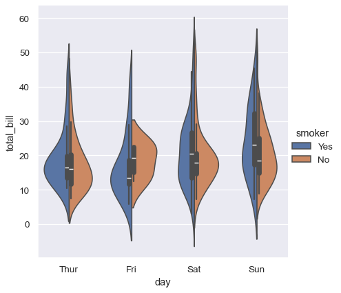
Alternately, you could use kernel density estimation to represent the underlying distribution that the points are sampled from:

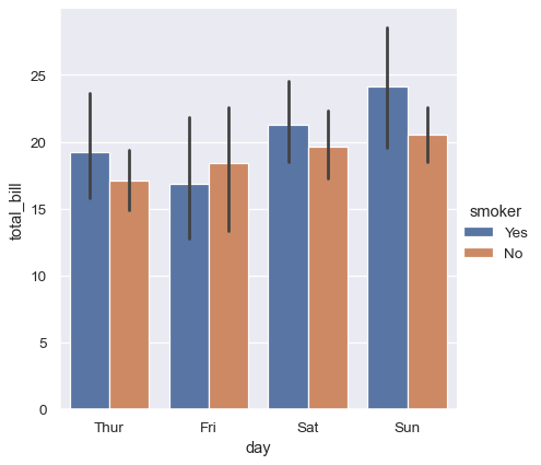
Or you could show only the mean value and its confidence interval within each nested category:

Multivariate views on complex datasets#

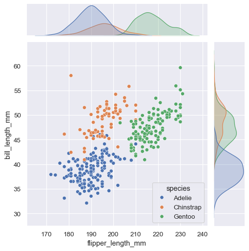
Some seaborn functions combine multiple kinds of plots to quickly give informative summaries of a dataset. One, jointplot() , focuses on a single relationship. It plots the joint distribution between two variables along with each variable’s marginal distribution:

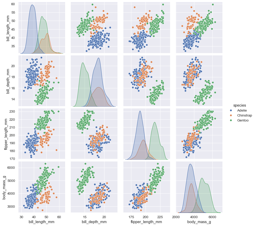
The other, pairplot() , takes a broader view: it shows joint and marginal distributions for all pairwise relationships and for each variable, respectively:

Lower-level tools for building figures#

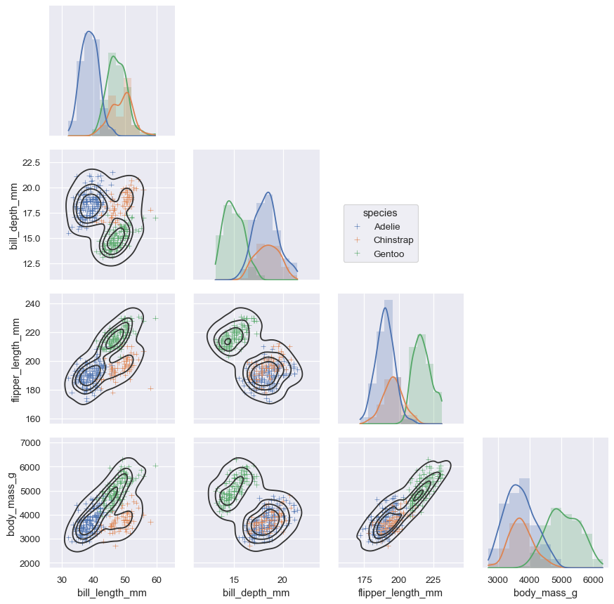
These tools work by combining axes-level plotting functions with objects that manage the layout of the figure, linking the structure of a dataset to a grid of axes . Both elements are part of the public API, and you can use them directly to create complex figures with only a few more lines of code:

Opinionated defaults and flexible customization#

Seaborn creates complete graphics with a single function call: when possible, its functions will automatically add informative axis labels and legends that explain the semantic mappings in the plot.

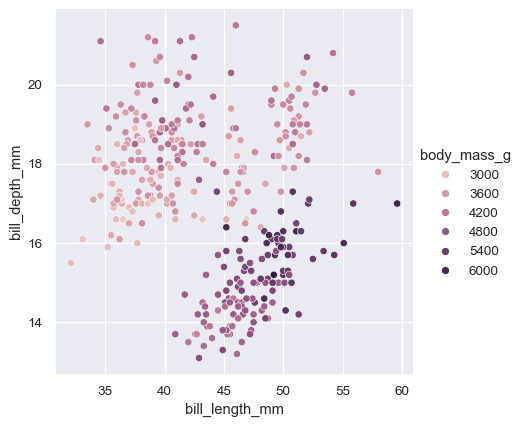
In many cases, seaborn will also choose default values for its parameters based on characteristics of the data. For example, the color mappings that we have seen so far used distinct hues (blue, orange, and sometimes green) to represent different levels of the categorical variables assigned to hue . When mapping a numeric variable, some functions will switch to a continuous gradient:

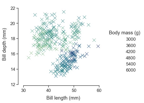
When you’re ready to share or publish your work, you’ll probably want to polish the figure beyond what the defaults achieve. Seaborn allows for several levels of customization. It defines multiple built-in themes that apply to all figures, its functions have standardized parameters that can modify the semantic mappings for each plot, and additional keyword arguments are passed down to the underlying matplotlib artists, allowing even more control. Once you’ve created a plot, its properties can be modified through both the seaborn API and by dropping down to the matplotlib layer for fine-grained tweaking:

Relationship to matplotlib#

Seaborn’s integration with matplotlib allows you to use it across the many environments that matplotlib supports, including exploratory analysis in notebooks, real-time interaction in GUI applications, and archival output in a number of raster and vector formats.

While you can be productive using only seaborn functions, full customization of your graphics will require some knowledge of matplotlib’s concepts and API. One aspect of the learning curve for new users of seaborn will be knowing when dropping down to the matplotlib layer is necessary to achieve a particular customization. On the other hand, users coming from matplotlib will find that much of their knowledge transfers.

Matplotlib has a comprehensive and powerful API; just about any attribute of the figure can be changed to your liking. A combination of seaborn’s high-level interface and matplotlib’s deep customizability will allow you both to quickly explore your data and to create graphics that can be tailored into a publication quality final product.

Next steps#

You have a few options for where to go next. You might first want to learn how to install seaborn . Once that’s done, you can browse the example gallery to get a broader sense for what kind of graphics seaborn can produce. Or you can read through the rest of the user guide and tutorial for a deeper discussion of the different tools and what they are designed to accomplish. If you have a specific plot in mind and want to know how to make it, you could check out the API reference , which documents each function’s parameters and shows many examples to illustrate usage.

Как строить красивые графики на Python с Seaborn

Визуализация данных — это метод, который позволяет специалистам по анализу данных преобразовывать сырые данные в диаграммы и графики, которые несут ценную информацию. Диаграммы уменьшают сложность данных и делают более понятными для любого пользователя.

Есть множество инструментов для визуализации данных, таких как Tableau, Power BI, ChartBlocks и других, которые являются no-code инструментами. Они очень мощные, и у каждого своя аудитория. Однако для работы с сырыми данными, требующими обработки, а также в качестве песочницы, Python подойдет лучше всего.

Несмотря на то, что этот путь сложнее и требует умения программировать, Python позволит вам провести любые манипуляции, преобразования и визуализировать ваши данные. Он идеально подходит для специалистов по анализу данных.

Python — лучший инструмент для data science и этому много причин, но самая важная — это его экосистема библиотек. Для работы с данными в Python есть много замечательных библиотек, таких как numpy , pandas , matplotlib , tensorflow .

Matplotlib , вероятно, самая известная библиотека для построения графиков, которая доступна в Python и других языках программирования, таких как R. Именно ее уровень кастомизации и удобства в использовании ставит ее на первое место. Однако с некоторыми действиями и кастомизациями во время ее использования бывает справиться нелегко.

Разработчики создали новую библиотеку на основе matplotlib , которая называется seaborn . Seaborn такая же мощная, как и matplotlib , но в то же время предоставляет большую абстракцию для упрощения графиков и привносит некоторые уникальные функции.

В этой статье мы сосредоточимся на том, как работать с seaborn для создания первоклассных графиков. Если хотите, можете создать новый проект и повторить все шаги или просто обратиться к моему руководству по seaborn на GitHub.

Что такое Seaborn?

Seaborn — это библиотека для создания статистических графиков на Python. Она основывается на matplotlib и тесно взаимодействует со структурами данных pandas.

Архитектура Seaborn позволяет вам быстро изучить и понять свои данные. Seaborn захватывает целые фреймы данных или массивы, в которых содержатся все ваши данные, и выполняет все внутренние функции, нужные для семантического маппинга и статистической агрегации для преобразования данных в информативные графики.

Она абстрагирует сложность, позволяя вам проектировать графики в соответствии с вашими нуждами.

Установка Seaborn

Установить seaborn так же просто, как и любую другую библиотеку, для этого вам понадобится ваш любимый менеджер пакетов Python. Во время установки seaborn библиотека установит все зависимости, включая matplotlib , pandas , numpy и scipy .

Давайте уже установим seaborn и, конечно же, также пакет notebook , чтобы получить доступ к песочнице с данными.

Помимо этого, перед началом работы давайте импортируем несколько модулей.

Строим первые графики

Перед тем, как мы начнем строить графики, нам нужны данные. Прелесть seaborn в том, что он работает непосредственно с объектами dataframe из pandas , что делает ее очень удобной. Более того, библиотека поставляется с некоторыми встроенными наборами данных, которые можно использовать прямо из кода, и не загружать файлы вручную.

Как строить графики в python seaborn

Data Visualization is the presentation of data in pictorial format. It is extremely important for Data Analysis, primarily because of the fantastic ecosystem of data-centric Python packages. And it helps to understand the data, however, complex it is, the significance of data by summarizing and presenting a huge amount of data in a simple and easy-to-understand format and helps communicate information clearly and effectively.

Pandas and Seaborn is one of those packages and makes importing and analyzing data much easier. In this article, we will use Pandas and Seaborn to analyze data.

Pandas

Pandas offer tools for cleaning and process your data. It is the most popular Python library that is used for data analysis. In pandas, a data table is called a dataframe.

So, let’s start with creating Pandas data frame:

Example 1:

Python3

Output:

Example 2: load the CSV data from the system and display it through pandas.

Python3

Output:

Seaborn

Seaborn is an amazing visualization library for statistical graphics plotting in Python. It is built on the top of matplotlib library and also closely integrated into the data structures from pandas.

Installation

For python environment :

For conda environment :

Let’s create Some basic plots using seaborn:

Python3

Output:

Seaborn: statistical data visualization

Seaborn helps to visualize the statistical relationships, To understand how variables in a dataset are related to one another and how that relationship is dependent on other variables, we perform statistical analysis. This Statistical analysis helps to visualize the trends and identify various patterns in the dataset.

These are the plot will help to visualize:

• Line Plot
• Scatter Plot
• Box plot
• Point plot
• Count plot
• Violin plot
• Swarm plot
• Bar plot
• KDE Plot

Line plot:

Lineplot Is the most popular plot to draw a relationship between x and y with the possibility of several semantic groupings.

Syntax : sns.lineplot(x=None, y=None)

Parameters:

x, y: Input data variables; must be numeric. Can pass data directly or reference columns in data.

Let’s visualize the data with a line plot and pandas:

Example 1:

Python3

Output:

Example 2: Use the hue parameter for plotting the graph.

Python3

Output:

Scatter Plot:

Scatterplot Can be used with several semantic groupings which can help to understand well in a graph against continuous/categorical data. It can draw a two-dimensional graph.

Syntax: seaborn.scatterplot(x=None, y=None)

Parameters:
x, y: Input data variables that should be numeric.

Returns: This method returns the Axes object with the plot drawn onto it.

Let’s visualize the data with a scatter plot and pandas:

Example 1:

Python3

Output:

Example 2: Use the hue parameter for plotting the graph.

Python3

Output:

Box plot:

A box plot (or box-and-whisker plot) s is the visual representation of the depicting groups of numerical data through their quartiles against continuous/categorical data.

A box plot consists of 5 things.

• Minimum
• First Quartile or 25%
• Median (Second Quartile) or 50%
• Third Quartile or 75%
• Maximum

• x, y, hue: Inputs for plotting long-form data.
• data: Dataset for plotting. If x and y are absent, this is interpreted as wide-form.

Draw the box plot with Pandas:

Example 1:

Python3

Output:

Example 2:

Python3

Output:

Violin Plot:

A violin plot is similar to a boxplot. It shows several quantitative data across one or more categorical variables such that those distributions can be compared.

• x, y, hue: Inputs for plotting long-form data.
• data: Dataset for plotting.

Draw the violin plot with Pandas:

Example 1:

Python3

Output:

Example 2:

Python3

Output:

Swarm plot:

A swarm plot is similar to a strip plot, We can draw a swarm plot with non-overlapping points against categorical data.

• x, y, hue: Inputs for plotting long-form data.
• data: Dataset for plotting.

Draw the swarm plot with Pandas:

Example 1:

Python3

Output:

Example 2:

Python3

Output:

Bar plot:

Barplot represents an estimate of central tendency for a numeric variable with the height of each rectangle and provides some indication of the uncertainty around that estimate using error bars.

• x, y : This parameter take names of variables in data or vector data, Inputs for plotting long-form data.
• hue : (optional) This parameter take column name for colour encoding.
• data : (optional) This parameter take DataFrame, array, or list of arrays, Dataset for plotting. If x and y are absent, this is interpreted as wide-form. Otherwise it is expected to be long-form.

Draw the bar plot with Pandas:

Example 1:

Python3

Output:

Example 2:

Python3

Output:

Point plot:

Point plot used to show point estimates and confidence intervals using scatter plot glyphs. A point plot represents an estimate of central tendency for a numeric variable by the position of scatter plot points and provides some indication of the uncertainty around that estimate using error bars.

• x, y: Inputs for plotting long-form data.
• hue: (optional) column name for color encoding.
• data: dataframe as a Dataset for plotting.

Draw the point plot with Pandas:

Example:

Python3

Output:

Count plot:

Count plot used to Show the counts of observations in each categorical bin using bars.

• x, y: This parameter take names of variables in data or vector data, optional, Inputs for plotting long-form data.
• hue : (optional) This parameter take column name for color encoding.
• data : (optional) This parameter take DataFrame, array, or list of arrays, Dataset for plotting. If x and y are absent, this is interpreted as wide-form. Otherwise, it is expected to be long-form.

Draw the count plot with Pandas:

Example:

Python3

Output:

KDE Plot:

KDE Plot described as Kernel Density Estimate is used for visualizing the Probability Density of a continuous variable. It depicts the probability density at different values in a continuous variable. We can also plot a single graph for multiple samples which helps in more efficient data visualization.

Syntax: seaborn.kdeplot(x=None, *, y=None, vertical=False, palette=None, **kwargs)

Parameters:

x, y : vectors or keys in data

vertical : boolean (True or False)

data : pandas.DataFrame, numpy.ndarray, mapping, or sequence

Draw the KDE plot with Pandas:

Example 1:

Python3

Output:

Example 2:

Python3

Output:

Bivariate and Univariate data using seaborn and pandas:

Before starting let’s have a small intro of bivariate and univariate data:

Bivariate data: This type of data involves two different variables. The analysis of this type of data deals with causes and relationships and the analysis is done to find out the relationship between the two variables.

Univariate data: This type of data consists of only one variable. The analysis of univariate data is thus the simplest form of analysis since the information deals with only one quantity that changes. It does not deal with causes or relationships and the main purpose of the analysis is to describe the data and find patterns that exist within it.

Complete Seaborn Python Tutorial for Data Visualization in Python

Seaborn is a Python data visualization library based on matplotlib. It provides a high-level interface for drawing attractive and informative statistical graphics.

Statistical analysis is a process of understanding how variables in a dataset relate to each other and how those relationships depend on other variables. Visualization can be a core component of this process because, when data are visualized properly, the human visual system can see trends and patterns that indicate a relationship.

1. Numerical Data Plotting

• relplot()
• scatterplot()
• lineplot()

2. Categorical Data Ploting

• catplot()
• boxplot()
• stripplot()
• swarmplot()
• etc…

3. Visualizing Distribution of the Data

• distplot()
• kdeplot()
• jointplot()
• rugplot()

4. Linear Regression and Relationship

• regplot()
• lmplot()

5. Controlling Plotted Figure Aesthetics

• figure styling
• axes styling
• color palettes
• etc..

The necessary python libraries are imported here-

• seaborn is used to draw various types of graphs.
• numpy is used to perform basic array operations.
• pyplot from matplotlib is used to visualize the results.
• pandas is used to read and create the dataset.
• %matplotlib inline sets the backend of matplotlib to the ‘inline’ backend: With this backend, the output of plotting commands is displayed inline within frontends like the Jupyter notebook, directly below the code cell that produced it.

We are going to set the style to darkgrid .The grid helps the plot serve as a lookup table for quantitative information, and the white-on grey helps to keep the grid from competing with lines that represent data.

Now we are going to load the data using sns.load_dataset . Seaborn has some inbuilt dataset. tips is the one of them. tips.tail() displays the last 5 rows of the dataset

Now we will plot the relational plot using the sns.relplot and visualize the relation between total_bill and tip .

As you can see, the above plot is a FacetGrid . It is a class that maps a dataset onto multiple axes arrayed in a grid of rows and columns that correspond to levels of variables in the dataset. Below is a list of things we can apply on FacetGrid .

value_counts return a Series containing counts of unique values. Here we will get the total number of non-smokers and the total number of smokers.

Here we have included smoker and time as well. hue groups variable that will produce elements with different colors. style groups variable that will produce elements with different styles.

Here we have used style for the size variable.

Earlier we have used hue for categorical values i.e. for smoker . Now we will use hue for numerical values i.e. for size . We can change the palette using cubehelix .

size groups variable that will produce elements with different sizes.

sizes is an object that determines how sizes are chosen when size is used. Here the smallest circle will be of size 15. The largest circle will be of size 200 and all the others will lie in between.

Now we will generate a new dataset to plot a lineplot . np.arange() returns an array with evenly spaced elements. Here it will return values from 0 to 499. randn() returns an array of defined shape, filled with random floating-point samples from the standard normal distribution. Here we will get an array of 500 random values. cumsum() gives the cumulative sum value.

By using kind we can change the kind of plot drawn. By default, it is set to scatter . Now we will change it to line .

In the above data, the values in time are sorted. Let's see what happens if the values are not sorted. For this, we will create a new dataset.

Below we have drawn the plot with unsorted values of the time. You can even draw the plot with sorted values of time by setting sort = True which will sort the values of the x-axis.

Now we will load the fmri dataset.

As you can see in the dataset same values timepoint have different corresponding values of signal . If we draw such a plot we get a confidence interval with 95% confidence. To remove the confidence interval we can set ci = False

We can also have ci = 'sd' to get the standard deviation in the plot.

If we want to plot data without any confidence interval we can set estimator = None . This will plot the real dataset.

Now we can add a third variable using hue = 'event' .

Here we have used 4 variables by setting hue = 'region' and style = 'event' .

We can improve the plots by placing markers on the data points by including markers = True . We can also remove the dash lines by including dashes = False .

We can even set hue and style to the same variable to emphasize more and make the plots more informative.

We can set units = subject so that each subject will have a separate line in the plot. While selecting the data we can give a condition using fmri.query() . Here we have given the condition that the value of event should be stim .

Now we will load the dataset dots using a condition.

We can set the colour pallete by using sns.cubehelix_pallete . We can set the number of colors in the palette using n_colors . We can specify the intensity of the lightest color in the palette using light .

We can even change the width of the lines based on some value using size . As we have set size = 'choice' the width of the line will change according to the value of choice . We can even add sizes to set the width.

Now we will see how to plot different kinds of non-numerical data such as dates. For that, we will generate a new dataset. pd.date_range() returns a fixed frequency DatetimeIndex . periods specifies the number of periods to generate.

g is an object which contains the FacetGrid returned by sns.relplot() . fig.autofmt_xdate() formats the dates.

Using FacetGrid we can plot multiple plots simultaneously. Using col we can specify the categorical variables that will determine the faceting of the grid. Here col = 'time' so we are getting two plots for lunch and dinner separately.

Here col = 'size' so we are getting 6 plots for all the sizes separately

Now we can plot a 2×2 FacetGrid using row and col . By using height we can set the height (in inches) of each facet.

col_wrap wraps the column variable at the given width, so that the column facets span multiple rows.

We can also plot line plots using sns.lineplot() .

We can plot scatter plots using sns.scatterplot() .

Now we will use sns.lineplot . Here we have set ci = 68 and we have shown the error using bars by setting err_style='bars' .The size of confidence intervals to draw around estimated values is 68.

Here we have plotted subject separately and we have used a single region i.e. 'frontal' . We can specify the line weight using lw .

Now let's work with scatter plots .

Now we are going to load the iris dataset .

Instead of passing the data = iris we can even set x and y in the way shown below.

2. Categorical Data Plotting

• catplot()
• boxplot()
• stripplot()
• swarmplot()
• etc…

Now we will see how to plot categorical data.

Here day has categorical data and total_bill has numerical data .

We can even interchange the variables on x and y axis to get a horizontal catplot plot.

The jitter parameter controls the magnitude of jitter or disables it altogether. Here we have disable the jitter.

In catplot() we can set the kind parameter to swarm to avoid overlap of points.

We can set the order in which categorical values should be plotted using order . By default categorical levels are inferred from the data objects.

If we want detailed characteristics of data we can use box plot by setting kind = 'box' .

Box plots show the five-number summary of a set of data: including the minimum, first (lower) quartile, median, third (upper) quartile, and maximum.

dodge = False merges the box plots of categorical values

Now we will load the diamonds dataset.

If you want more visualize detailed information you can use boxen plot . It is similar to a box plot in plotting a nonparametric representation of a distribution in which all features correspond to actual observations. By plotting more quantiles, it provides more information about the shape of the distribution, particularly in the tails. While giving the data we are sorting the data according to the colour using diamonds.sort_values('color') .

Violin plot shows the distribution of quantitative data across several levels of one (or more) categorical variables such that those distributions can be compared. Unlike a box plot, in which all of the plot components correspond to actual data points, the violin plot features a kernel density estimation of the underlying distribution.

We can draw a violin plot by setting kind = 'violin' . When using hue nesting with a variable that takes two levels, setting split to True will draw half of a violin for each level. This can make it easier to directly compare the distributions.

Now we will draw the violin plot and swarm plot together.

inner = None enables representation of the datapoints in the violin interior. The value of parameter ax represents the axes object to draw the plot onto. Here we have set ax of swarmplot to g.ax which represents the violin plot.

Now we will load the titanic dataset.

We will now plot a barplot . The black line represents the probability of error.

Now we will plot a count plot . We can change the gradient of the colour using palette parameter.

A point plot represents an estimate of central tendency for a numeric variable by the position of scatter plot points and provides some indication of the uncertainty around that estimate using error bars.

3. Visualizing Distribution of the Data

• distplot()
• kdeplot()
• jointplot()
• rugplot()

We can plot univariate distribution using sns.distplot() . By default, this will draw a histogram and fit a kernel density estimate (KDE).

rug draws a small vertical tick at each observation. bins is the specification of hist bins.

Now lets plot a kdeplot .

shade = True shades in the area under the KDE curve. We can control the bandwidth using bw . The parameter cut draws the estimate to cut * bw from the extreme data points i.e. it cuts the plot and zooms it.

Now we will see how to plot bivariate distribution .

Now we will plot a joint plot . It displays relationship between 2 variables (bivariate) as well as 1D profiles (univariate) in the margins.

By using kind we can select the kind of plot to draw. Here we have selected kind = 'hex' .

subplots() returns the figure and axes.

sns.cubehelix_palette() produces a colormap with linearly-decreasing (or increasing) brightness. as_cmap = True returns a matplotlib colormap instead of a list of colors. The intensity of the darkest and ligtest colours in the palette can be controlled by dark and light . As reverse = True the palette will go from dark to light.

sns.kdeplot will plot a kde plot. shade = True shades in the area under the KDE curve.

The jointplot() function uses a JointGrid to manage the figure. For more flexibility, you may want to draw your figure by using JointGrid directly. jointplot() returns the JointGrid object after plotting, which you can use to add more layers or to tweak other aspects of the visualization.

sns.plot_joint() draws a bivariate plot of x and y. c and s parameters are for colour and size respectively.

We aew going to join the x axis using collections and control the transparency using set_alpha()

Now we will draw pair plots using sns.pairplot() .By default, this function will create a grid of Axes such that each numeric variable in data will by shared in the y-axis across a single row and in the x-axis across a single column. The diagonal Axes are treated differently, drawing a plot to show the univariate distribution of the data for the variable in that column.

map_diag() draws the diagonal elements are plotted as a kde plot . map_offdiag() draws the non-diagonal elements as a kde plot with number of levels = 10.

4. Linear Regression and Relationship

• regplot()
• lmplot()

We can draw regression plots with the help of sns.regplot() . The plot drawn below shows the relationship between total_bill and tip .

We can draw a linear model plot using sns.lmplot() .

We can draw a plot which shows the linear relationship between size and tips .

If we set x_estimator = np.mean the dots in the above plot will be replaced by the mean and a confidence line.

Now we will see how to draw a plot for the data which is not linearly related. To do this we will load the anscombe dataset.

This dataset contains 4 types of data and each type contains 11 values.

Now we will draw a plot for the data of type I from the dataset. scatter_kws is used to pass additional keyword arguments.

Now we will plot the dataset type II. We can see that it is not a linear relation. In order to fit such type of dataset, we can use the order parameter. If an order is greater than 1, it estimates a polynomial regression.

Now we will see how to handle outliers . An outlier is a data point that differs significantly from other observations. We can go and manually remove the outlier from the dataset or we can set robust = True to nullify its effect while drawing the plot.

We can change the size of figure using subplots() and pass the parameter figsize .

We can even control the height and the position of the plots using height and col_wrap .

5. Controlling Plotted Figure Aesthetics

• figure styling
• axes styling
• color palettes
• etc..

Here is a function to draw a sinplot .

sns.set_style() is used to set the aesthetic style of the plots. ticks will add ticks on the axes. 'axes.grid': True enables the grid in the background of the plot. 'xtick.direcyion': 'in' makes the ticks on the x axis to point inwards. sns.despine() removes the top and right spines from plot. left = True removes the left spine.

sns.axes_style() shows all the current elements which are set on the plot. We can change the values of these elements and customize our plots.

sns.set_context() sets the plotting context parameters. This affects things like the size of the labels, lines, and other elements of the plot, but not the overall style. The base context is “notebook”, and the other contexts are “paper”, “talk”, and “poster”, which are version of the notebook parameters scaled by .8, 1.3, and 1.6, respectively. We can even use font_scale which is a separate scaling factor to independently scale the size of the font elements.

Now we will see some colour palettes which seaborn uses. sns.color_palette() returns a list of the current colors defining a color palette.

We can use the the hls color space, which is a simple transformation of RGB values to create colour palettes.

Conclusion

• With the help of data visualization, we can see how the data looks like and what kind of correlation is held by the attributes of data.
• This is the first and foremost step where they will get a high-level statistical overview on how the data is and some of its attributes like the underlying distribution, presence of outliers, and several more useful features.
• From the perspective of building models, by visualizing the data we can find the hidden patterns, explore if there are any clusters within data and we can find if they are linearly separable/too much overlapped etc.
• From this initial analysis we can easily rule out the models that won’t be suitable for such data and we will implement only the models that are suitable, without wasting our valuable time and computational resources.

Further Reading

If you are looking for beginners to advanced courses on NLP. You can enroll in one of my best NLP courses on Udemy.