Validation Basics
This chapter focuses on the basics of model validation. From splitting data into training, validation, and testing datasets, to creating an understanding of the bias-variance tradeoff, we build the foundation for the techniques of K-Fold and Leave-One-Out validation practiced in chapter three. This is the Summary of lecture «Model Validation in Python», via datacamp.
Jul 13, 2020 • Chanseok Kang • 13 min read
Creating train,test, and validation datasets
- Traditional train/test split
- Seen data (used for training)
- Unseen data (unavailable for training)
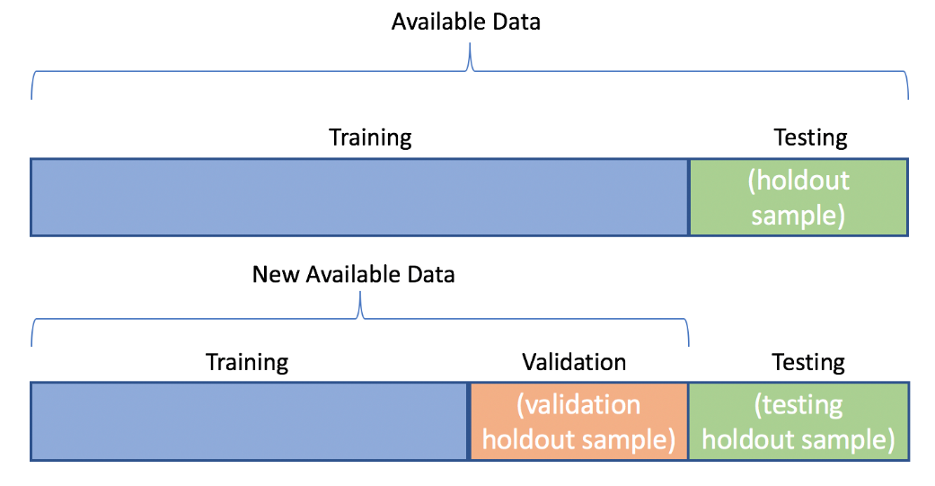
Create one holdout set
Your boss has asked you to create a simple random forest model on the tic_tac_toe dataset. She doesn’t want you to spend much time selecting parameters; rather she wants to know how well the model will perform on future data. For future Tic-Tac-Toe games, it would be nice to know if your model can predict which player will win.
Top-Left Top-Middle Top-Right Middle-Left Middle-Middle Middle-Right Bottom-Left Bottom-Middle Bottom-Right Class 0 x x x x o o x o o positive 1 x x x x o o o x o positive 2 x x x x o o o o x positive 3 x x x x o o o b b positive 4 x x x x o o b o b positive Create two holdout sets
You recently created a simple random forest model to predict Tic-Tac-Toe game wins for your boss, and at her request, you did not do any parameter tuning. Unfortunately, the overall model accuracy was too low for her standards. This time around, she has asked you to focus on model performance.
Before you start testing different models and parameter sets, you will need to split the data into training, validation, and testing datasets. Remember that after splitting the data into training and testing datasets, the validation dataset is created by splitting the training dataset.
You now have training, validation, and testing datasets, but do you know when you need both validation and testing datasets?
Accuracy metrics: regression models
- Mean absolute error (MAE) $$ \text
= \frac<\sum_ \vert y_i — \hat \vert> $$ - Simplest and most intuitive metric
- Treats all points equally
- Not sensitive to outliers
- Most widely used regression metric
- Allows outlier errors to contribute more to the overall error
- Random family road trips could lead to large errors in predictions
- Accuracy metrics are always application apecific
- MAE and MSE error terms are in different units and should not be compared
Mean absolute error
Communicating modeling results can be difficult. However, most clients understand that on average, a predictive model was off by some number. This makes explaining the mean absolute error easy. For example, when predicting the number of wins for a basketball team, if you predict 42, and they end up with 40, you can easily explain that the error was two wins.
In this exercise, you are interviewing for a new position and are provided with two arrays. y_test , the true number of wins for all 30 NBA teams in 2017 and predictions , which contains a prediction for each team. To test your understanding, you are asked to both manually calculate the MAE and use sklearn .
Standard assumptions for regression analysis
This assumption implies that there should be linear relationship between the response variables and the predictor. Checking the linearity assumption may require plotting of predictor versus response variables.
As shown in Figure 1 above, This should be fairly easy for simple linear regression but in multiple linear regression with large number of predictor variables, we can use standardised residual plot against each one of the predictor variables. The ideal plot of residuals with each of the predictor should be a random scatter because we assume that the residuals are uncorrelated with the predictor variables. Any noticeable pattern in such plots indicates violation of linear relationship assumption.
Let us try to plot residuals with a predictor variable X1 in the given data set as described below. This dataset has many other predictor variables named X2, X3 and so on, but for the sake of simplicity we are performing the plot only for one predictor X1.
We have calculated the residual array in the code snippet above. Now we will plot this residual with X1 predictor.
The residual plot is shown in the figure 2 below. As we can see that plot is not a random scatter plot instead this plot is forming a curve. A plot like this is indicating the non-linearity.
Handling non-linearity problem
When the linear relationship does not hold we can either transform the data variables like log, exponential transformation or normalisation etc, as shown in previous parts. Also in such cases we can try to use suitable non linear regression models as well. Non linear regression models will be discussed in next parts.2. predictor variable should be linearly independent
One more assumption for standard regression is that predictor variables should be linearly independent of each other. If they won’t be linearly independent then the uniqueness of the least squares solution can not be assured. This problem is also called as collinearity or multicollinearity. In this situation strong correlations exist between among the predictor variables which may cause the erroneous estimates of the coefficients. It also impacts the stability of coefficient estimates as their values can change erroneously even on a slight changes in model specification. Multicollinearity does not affect the predictive power but individual predictor variable’s impact on the response variable could be calculated wrongly.
Longley dataset available in stats model is known to possess big multicollinearity. We will use this data in our experiment below.
The warning about the condition number above indicates the strong multicollinearity. If values of condition number are very large then we can say that multicollinearity may be there. Condition number can be computed using eigen values of normalised predictor variable.
Also we can predict multicollinearity by directly looking at the eigen vector of a correlation matrix.
If at least one of the eigen values of the correlation matrix is close to zero then we can say that multicollinearity exists in the dataset. In the code snippet above we can see multiple values are very much close to zero. An almost zero eigen value shows minimal variation in the data orthogonal with other eigen vectors.
Handling multicollinearity
There are several measures to handle the multicollinearity but to keep it brief we are listing down only the most popular and widely used methods.- We can try to remove the variables causing the multicollinearity in our dataset. Lets consider the eigen vectors generated in the example above.
The eigen values at index 3,4 and 5 are close to zero. There corresponding eigen vectors are:
Now we ignore the columns with values consistently close to zero in each of the selected eigen vectors. In the output produced above, column index 2 and 3 have near zero values in all three eigen vectors so we can say that columns 0,1,4 and 5 are strongly correlated with each other so any one of them would be sufficient to capture the essence of the other three columns.
We can see that after removing correlated columns none of the eigen value is very much close to zero as in the case earlier.
2. we can perform the regression on latent variables provided by some data compression method like PCA or we can use partial least squares method. Partial least squares regression method obtains a linear regression model by projecting the predicted variables and the predictors to a new space.
3. We can leave the model as it based on our use case of course, because the problem of multicollinearity does not affect the predicting power of a model if the predictor variables follow the same collinearity pattern in the new data used for prediction.
3.3. Metrics and scoring: quantifying the quality of predictions
There are 3 different APIs for evaluating the quality of a model’s predictions:
Estimator score method: Estimators have a score method providing a default evaluation criterion for the problem they are designed to solve. This is not discussed on this page, but in each estimator’s documentation.
Scoring parameter: Model-evaluation tools using cross-validation (such as model_selection.cross_val_score and model_selection.GridSearchCV ) rely on an internal scoring strategy. This is discussed in the section The scoring parameter: defining model evaluation rules .
Metric functions: The sklearn.metrics module implements functions assessing prediction error for specific purposes. These metrics are detailed in sections on Classification metrics , Multilabel ranking metrics , Regression metrics and Clustering metrics .
Finally, Dummy estimators are useful to get a baseline value of those metrics for random predictions.
For “pairwise” metrics, between samples and not estimators or predictions, see the Pairwise metrics, Affinities and Kernels section.
3.3.1. The scoring parameter: defining model evaluation rules
Model selection and evaluation using tools, such as model_selection.GridSearchCV and model_selection.cross_val_score , take a scoring parameter that controls what metric they apply to the estimators evaluated.
3.3.1.1. Common cases: predefined values
For the most common use cases, you can designate a scorer object with the scoring parameter; the table below shows all possible values. All scorer objects follow the convention that higher return values are better than lower return values. Thus metrics which measure the distance between the model and the data, like metrics.mean_squared_error , are available as neg_mean_squared_error which return the negated value of the metric.
Classification
for binary targets
by multilabel sample
requires predict_proba support
suffixes apply as with ‘f1’
suffixes apply as with ‘f1’
suffixes apply as with ‘f1’
Clustering
Regression
The values listed by the ValueError exception correspond to the functions measuring prediction accuracy described in the following sections. You can retrieve the names of all available scorers by calling get_scorer_names .
3.3.1.2. Defining your scoring strategy from metric functions
The module sklearn.metrics also exposes a set of simple functions measuring a prediction error given ground truth and prediction:
functions ending with _score return a value to maximize, the higher the better.
functions ending with _error or _loss return a value to minimize, the lower the better. When converting into a scorer object using make_scorer , set the greater_is_better parameter to False ( True by default; see the parameter description below).
Metrics available for various machine learning tasks are detailed in sections below.
Many metrics are not given names to be used as scoring values, sometimes because they require additional parameters, such as fbeta_score . In such cases, you need to generate an appropriate scoring object. The simplest way to generate a callable object for scoring is by using make_scorer . That function converts metrics into callables that can be used for model evaluation.
One typical use case is to wrap an existing metric function from the library with non-default values for its parameters, such as the beta parameter for the fbeta_score function:
The second use case is to build a completely custom scorer object from a simple python function using make_scorer , which can take several parameters:
the python function you want to use ( my_custom_loss_func in the example below)
whether the python function returns a score ( greater_is_better=True , the default) or a loss ( greater_is_better=False ). If a loss, the output of the python function is negated by the scorer object, conforming to the cross validation convention that scorers return higher values for better models.
for classification metrics only: whether the python function you provided requires continuous decision certainties ( needs_threshold=True ). The default value is False.
any additional parameters, such as beta or labels in f1_score .
Here is an example of building custom scorers, and of using the greater_is_better parameter:
3.3.1.3. Implementing your own scoring object
You can generate even more flexible model scorers by constructing your own scoring object from scratch, without using the make_scorer factory. For a callable to be a scorer, it needs to meet the protocol specified by the following two rules:
It can be called with parameters (estimator, X, y) , where estimator is the model that should be evaluated, X is validation data, and y is the ground truth target for X (in the supervised case) or None (in the unsupervised case).
It returns a floating point number that quantifies the estimator prediction quality on X , with reference to y . Again, by convention higher numbers are better, so if your scorer returns loss, that value should be negated.
Using custom scorers in functions where n_jobs > 1
While defining the custom scoring function alongside the calling function should work out of the box with the default joblib backend (loky), importing it from another module will be a more robust approach and work independently of the joblib backend.
For example, to use n_jobs greater than 1 in the example below, custom_scoring_function function is saved in a user-created module ( custom_scorer_module.py ) and imported:
3.3.1.4. Using multiple metric evaluation
Scikit-learn also permits evaluation of multiple metrics in GridSearchCV , RandomizedSearchCV and cross_validate .
There are three ways to specify multiple scoring metrics for the scoring parameter:
-
As an iterable of string metrics::
Note that the dict values can either be scorer functions or one of the predefined metric strings.
As a callable that returns a dictionary of scores:
3.3.2. Classification metrics
The sklearn.metrics module implements several loss, score, and utility functions to measure classification performance. Some metrics might require probability estimates of the positive class, confidence values, or binary decisions values. Most implementations allow each sample to provide a weighted contribution to the overall score, through the sample_weight parameter.
Some of these are restricted to the binary classification case:
Compute precision-recall pairs for different probability thresholds.
roc_curve (y_true, y_score, *[, pos_label, . ])
Compute Receiver operating characteristic (ROC).
Compute binary classification positive and negative likelihood ratios.
det_curve (y_true, y_score[, pos_label, . ])
Compute error rates for different probability thresholds.
Others also work in the multiclass case:
Compute the balanced accuracy.
Compute Cohen’s kappa: a statistic that measures inter-annotator agreement.
Compute confusion matrix to evaluate the accuracy of a classification.
Average hinge loss (non-regularized).
Compute the Matthews correlation coefficient (MCC).
Compute Area Under the Receiver Operating Characteristic Curve (ROC AUC) from prediction scores.
Top-k Accuracy classification score.
Some also work in the multilabel case:
Accuracy classification score.
Build a text report showing the main classification metrics.
Compute the F1 score, also known as balanced F-score or F-measure.
Compute the F-beta score.
hamming_loss (y_true, y_pred, *[, sample_weight])
Compute the average Hamming loss.
Jaccard similarity coefficient score.
Log loss, aka logistic loss or cross-entropy loss.
Compute a confusion matrix for each class or sample.
Compute precision, recall, F-measure and support for each class.
Compute the precision.
Compute the recall.
Compute Area Under the Receiver Operating Characteristic Curve (ROC AUC) from prediction scores.
Zero-one classification loss.
And some work with binary and multilabel (but not multiclass) problems:
Compute average precision (AP) from prediction scores.
In the following sub-sections, we will describe each of those functions, preceded by some notes on common API and metric definition.
3.3.2.1. From binary to multiclass and multilabel
Some metrics are essentially defined for binary classification tasks (e.g. f1_score , roc_auc_score ). In these cases, by default only the positive label is evaluated, assuming by default that the positive class is labelled 1 (though this may be configurable through the pos_label parameter).
In extending a binary metric to multiclass or multilabel problems, the data is treated as a collection of binary problems, one for each class. There are then a number of ways to average binary metric calculations across the set of classes, each of which may be useful in some scenario. Where available, you should select among these using the average parameter.
"macro" simply calculates the mean of the binary metrics, giving equal weight to each class. In problems where infrequent classes are nonetheless important, macro-averaging may be a means of highlighting their performance. On the other hand, the assumption that all classes are equally important is often untrue, such that macro-averaging will over-emphasize the typically low performance on an infrequent class.
"weighted" accounts for class imbalance by computing the average of binary metrics in which each class’s score is weighted by its presence in the true data sample.
"micro" gives each sample-class pair an equal contribution to the overall metric (except as a result of sample-weight). Rather than summing the metric per class, this sums the dividends and divisors that make up the per-class metrics to calculate an overall quotient. Micro-averaging may be preferred in multilabel settings, including multiclass classification where a majority class is to be ignored.
"samples" applies only to multilabel problems. It does not calculate a per-class measure, instead calculating the metric over the true and predicted classes for each sample in the evaluation data, and returning their ( sample_weight -weighted) average.
Selecting average=None will return an array with the score for each class.
While multiclass data is provided to the metric, like binary targets, as an array of class labels, multilabel data is specified as an indicator matrix, in which cell [i, j] has value 1 if sample i has label j and value 0 otherwise.
3.3.2.2. Accuracy score
The accuracy_score function computes the accuracy, either the fraction (default) or the count (normalize=False) of correct predictions.
In multilabel classification, the function returns the subset accuracy. If the entire set of predicted labels for a sample strictly match with the true set of labels, then the subset accuracy is 1.0; otherwise it is 0.0.
If \(\hat
_i\) is the predicted value of the \(i\) -th sample and \(y_i\) is the corresponding true value, then the fraction of correct predictions over \(n_\text \) is defined as In the multilabel case with binary label indicators:
See Test with permutations the significance of a classification score for an example of accuracy score usage using permutations of the dataset.
3.3.2.3. Top-k accuracy score
The top_k_accuracy_score function is a generalization of accuracy_score . The difference is that a prediction is considered correct as long as the true label is associated with one of the k highest predicted scores. accuracy_score is the special case of k = 1 .
The function covers the binary and multiclass classification cases but not the multilabel case.
If \(\hat
_ \) is defined as where \(k\) is the number of guesses allowed and \(1(x)\) is the indicator function.
3.3.2.4. Balanced accuracy score
The balanced_accuracy_score function computes the balanced accuracy, which avoids inflated performance estimates on imbalanced datasets. It is the macro-average of recall scores per class or, equivalently, raw accuracy where each sample is weighted according to the inverse prevalence of its true class. Thus for balanced datasets, the score is equal to accuracy.
In the binary case, balanced accuracy is equal to the arithmetic mean of sensitivity (true positive rate) and specificity (true negative rate), or the area under the ROC curve with binary predictions rather than scores:
If the classifier performs equally well on either class, this term reduces to the conventional accuracy (i.e., the number of correct predictions divided by the total number of predictions).
In contrast, if the conventional accuracy is above chance only because the classifier takes advantage of an imbalanced test set, then the balanced accuracy, as appropriate, will drop to \(\frac<1>
The score ranges from 0 to 1, or when adjusted=True is used, it rescaled to the range \(\frac<1><1 - n\_classes>\) to 1, inclusive, with performance at random scoring 0.
If \(y_i\) is the true value of the \(i\) -th sample, and \(w_i\) is the corresponding sample weight, then we adjust the sample weight to:
where \(1(x)\) is the indicator function. Given predicted \(\hat
_i\) for sample \(i\) , balanced accuracy is defined as: With adjusted=True , balanced accuracy reports the relative increase from \(\texttt
(y, \mathbf<0>, w) = \frac<1> The multiclass definition here seems the most reasonable extension of the metric used in binary classification, though there is no certain consensus in the literature:
Our definition: [Mosley2013] , [Kelleher2015] and [Guyon2015] , where [Guyon2015] adopt the adjusted version to ensure that random predictions have a score of \(0\) and perfect predictions have a score of \(1\) ..
Class balanced accuracy as described in [Mosley2013] : the minimum between the precision and the recall for each class is computed. Those values are then averaged over the total number of classes to get the balanced accuracy.
Balanced Accuracy as described in [Urbanowicz2015] : the average of sensitivity and specificity is computed for each class and then averaged over total number of classes.
I. Guyon, K. Bennett, G. Cawley, H.J. Escalante, S. Escalera, T.K. Ho, N. Macià, B. Ray, M. Saeed, A.R. Statnikov, E. Viegas, Design of the 2015 ChaLearn AutoML Challenge, IJCNN 2015.
3.3.2.5. Cohen’s kappa
The function cohen_kappa_score computes Cohen’s kappa statistic. This measure is intended to compare labelings by different human annotators, not a classifier versus a ground truth.
The kappa score (see docstring) is a number between -1 and 1. Scores above .8 are generally considered good agreement; zero or lower means no agreement (practically random labels).
Kappa scores can be computed for binary or multiclass problems, but not for multilabel problems (except by manually computing a per-label score) and not for more than two annotators.
3.3.2.6. Confusion matrix
The confusion_matrix function evaluates classification accuracy by computing the confusion matrix with each row corresponding to the true class (Wikipedia and other references may use different convention for axes).
By definition, entry \(i, j\) in a confusion matrix is the number of observations actually in group \(i\) , but predicted to be in group \(j\) . Here is an example:
ConfusionMatrixDisplay can be used to visually represent a confusion matrix as shown in the Confusion matrix example, which creates the following figure:
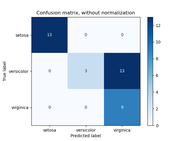
The parameter normalize allows to report ratios instead of counts. The confusion matrix can be normalized in 3 different ways: ‘pred’ , ‘true’ , and ‘all’ which will divide the counts by the sum of each columns, rows, or the entire matrix, respectively.
For binary problems, we can get counts of true negatives, false positives, false negatives and true positives as follows:
See Confusion matrix for an example of using a confusion matrix to evaluate classifier output quality.
See Recognizing hand-written digits for an example of using a confusion matrix to classify hand-written digits.
See Classification of text documents using sparse features for an example of using a confusion matrix to classify text documents.
3.3.2.7. Classification report
The classification_report function builds a text report showing the main classification metrics. Here is a small example with custom target_names and inferred labels:
See Recognizing hand-written digits for an example of classification report usage for hand-written digits.
See Custom refit strategy of a grid search with cross-validation for an example of classification report usage for grid search with nested cross-validation.
3.3.2.8. Hamming loss
The hamming_loss computes the average Hamming loss or Hamming distance between two sets of samples.
If \(\hat
_ \) is the number of samples and \(n_\text \) is the number of labels, then the Hamming loss \(L_ \) is defined as: The equation above does not hold true in the case of multiclass classification. Please refer to the note below for more information.
In the multilabel case with binary label indicators:
In multiclass classification, the Hamming loss corresponds to the Hamming distance between y_true and y_pred which is similar to the Zero one loss function. However, while zero-one loss penalizes prediction sets that do not strictly match true sets, the Hamming loss penalizes individual labels. Thus the Hamming loss, upper bounded by the zero-one loss, is always between zero and one, inclusive; and predicting a proper subset or superset of the true labels will give a Hamming loss between zero and one, exclusive.
3.3.2.9. Precision, recall and F-measures
Intuitively, precision is the ability of the classifier not to label as positive a sample that is negative, and recall is the ability of the classifier to find all the positive samples.
The F-measure ( \(F_\beta\) and \(F_1\) measures) can be interpreted as a weighted harmonic mean of the precision and recall. A \(F_\beta\) measure reaches its best value at 1 and its worst score at 0. With \(\beta = 1\) , \(F_\beta\) and \(F_1\) are equivalent, and the recall and the precision are equally important.
The precision_recall_curve computes a precision-recall curve from the ground truth label and a score given by the classifier by varying a decision threshold.
The average_precision_score function computes the average precision (AP) from prediction scores. The value is between 0 and 1 and higher is better. AP is defined as
where \(P_n\) and \(R_n\) are the precision and recall at the nth threshold. With random predictions, the AP is the fraction of positive samples.
References [Manning2008] and [Everingham2010] present alternative variants of AP that interpolate the precision-recall curve. Currently, average_precision_score does not implement any interpolated variant. References [Davis2006] and [Flach2015] describe why a linear interpolation of points on the precision-recall curve provides an overly-optimistic measure of classifier performance. This linear interpolation is used when computing area under the curve with the trapezoidal rule in auc .
Several functions allow you to analyze the precision, recall and F-measures score:
Compute average precision (AP) from prediction scores.
Compute the F1 score, also known as balanced F-score or F-measure.
Compute the F-beta score.
Compute precision-recall pairs for different probability thresholds.
Compute precision, recall, F-measure and support for each class.
Compute the precision.
Compute the recall.
Note that the precision_recall_curve function is restricted to the binary case. The average_precision_score function works only in binary classification and multilabel indicator format. The PredictionRecallDisplay.from_estimator and PredictionRecallDisplay.from_predictions functions will plot the precision-recall curve as follows.
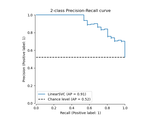
See Custom refit strategy of a grid search with cross-validation for an example of precision_score and recall_score usage to estimate parameters using grid search with nested cross-validation.
See Precision-Recall for an example of precision_recall_curve usage to evaluate classifier output quality.
M. Everingham, L. Van Gool, C.K.I. Williams, J. Winn, A. Zisserman, The Pascal Visual Object Classes (VOC) Challenge, IJCV 2010.
3.3.2.9.1. Binary classification
In a binary classification task, the terms ‘’positive’’ and ‘’negative’’ refer to the classifier’s prediction, and the terms ‘’true’’ and ‘’false’’ refer to whether that prediction corresponds to the external judgment (sometimes known as the ‘’observation’’). Given these definitions, we can formulate the following table:
Actual class (observation)
Predicted class (expectation)
tp (true positive) Correct result
fp (false positive) Unexpected result
fn (false negative) Missing result
tn (true negative) Correct absence of result
In this context, we can define the notions of precision, recall and F-measure:
Sometimes recall is also called ‘’sensitivity’’.
Here are some small examples in binary classification:
3.3.2.9.2. Multiclass and multilabel classification
In a multiclass and multilabel classification task, the notions of precision, recall, and F-measures can be applied to each label independently. There are a few ways to combine results across labels, specified by the average argument to the average_precision_score (multilabel only), f1_score , fbeta_score , precision_recall_fscore_support , precision_score and recall_score functions, as described above . Note that if all labels are included, “micro”-averaging in a multiclass setting will produce precision, recall and \(F\) that are all identical to accuracy. Also note that “weighted” averaging may produce an F-score that is not between precision and recall.
To make this more explicit, consider the following notation:
\(y\) the set of true \((sample, label)\) pairs
\(\hat
\) the set of predicted \((sample, label)\) pairs \(L\) the set of labels
\(S\) the set of samples
\(y_s\) the subset of \(y\) with sample \(s\) , i.e. \(y_s := \left\<(s', l) \in y | s' = s\right\>\)
\(y_l\) the subset of \(y\) with label \(l\)
similarly, \(\hat
_s\) and \(\hat _l\) are subsets of \(\hat \) \(R(A, B) := \frac<\left| A \cap B \right|><\left|A\right|>\) (Conventions vary on handling \(A = \emptyset\) ; this implementation uses \(R(A, B):=0\) , and similar for \(P\) .)
Then the metrics are defined as:
\(\frac<1> <\sum_
\left|y_l\right|> \sum_ \left|y_l\right| F_\beta(y_l, \hat _l)\) \(\langle P(y_l, \hat
_l) | l \in L \rangle\) \(\langle R(y_l, \hat
_l) | l \in L \rangle\) \(\langle F_\beta(y_l, \hat
_l) | l \in L \rangle\) For multiclass classification with a “negative class”, it is possible to exclude some labels:
Similarly, labels not present in the data sample may be accounted for in macro-averaging.
3.3.2.10. Jaccard similarity coefficient score
The jaccard_score function computes the average of Jaccard similarity coefficients, also called the Jaccard index, between pairs of label sets.
The Jaccard similarity coefficient with a ground truth label set \(y\) and predicted label set \(\hat
\) , is defined as The jaccard_score (like precision_recall_fscore_support ) applies natively to binary targets. By computing it set-wise it can be extended to apply to multilabel and multiclass through the use of average (see above ).
In the binary case:
In the 2D comparison case (e.g. image similarity):
In the multilabel case with binary label indicators:
Multiclass problems are binarized and treated like the corresponding multilabel problem:
3.3.2.11. Hinge loss
The hinge_loss function computes the average distance between the model and the data using hinge loss, a one-sided metric that considers only prediction errors. (Hinge loss is used in maximal margin classifiers such as support vector machines.)
If the true label \(y_i\) of a binary classification task is encoded as \(y_i=\left\<-1, +1\right\>\) for every sample \(i\) ; and \(w_i\) is the corresponding predicted decision (an array of shape ( n_samples ,) as output by the decision_function method), then the hinge loss is defined as:
If there are more than two labels, hinge_loss uses a multiclass variant due to Crammer & Singer. Here is the paper describing it.
In this case the predicted decision is an array of shape ( n_samples , n_labels ). If \(w_
_ y_j \ne y_i \right\>\) is the maximum of the predicted decisions for all the other labels, then the multi-class hinge loss is defined by:
Here is a small example demonstrating the use of the hinge_loss function with a svm classifier in a binary class problem:
Here is an example demonstrating the use of the hinge_loss function with a svm classifier in a multiclass problem:
3.3.2.12. Log loss
Log loss, also called logistic regression loss or cross-entropy loss, is defined on probability estimates. It is commonly used in (multinomial) logistic regression and neural networks, as well as in some variants of expectation-maximization, and can be used to evaluate the probability outputs ( predict_proba ) of a classifier instead of its discrete predictions.
For binary classification with a true label \(y \in \<0,1\>\) and a probability estimate \(p = \operatorname
(y = 1)\) , the log loss per sample is the negative log-likelihood of the classifier given the true label: This extends to the multiclass case as follows. Let the true labels for a set of samples be encoded as a 1-of-K binary indicator matrix \(Y\) , i.e., \(y_
(y_ To see how this generalizes the binary log loss given above, note that in the binary case, \(p_
The log_loss function computes log loss given a list of ground-truth labels and a probability matrix, as returned by an estimator’s predict_proba method.
The first [.9, .1] in y_pred denotes 90% probability that the first sample has label 0. The log loss is non-negative.
3.3.2.13. Matthews correlation coefficient
The matthews_corrcoef function computes the Matthew’s correlation coefficient (MCC) for binary classes. Quoting Wikipedia:
“The Matthews correlation coefficient is used in machine learning as a measure of the quality of binary (two-class) classifications. It takes into account true and false positives and negatives and is generally regarded as a balanced measure which can be used even if the classes are of very different sizes. The MCC is in essence a correlation coefficient value between -1 and +1. A coefficient of +1 represents a perfect prediction, 0 an average random prediction and -1 an inverse prediction. The statistic is also known as the phi coefficient.”
In the binary (two-class) case, \(tp\) , \(tn\) , \(fp\) and \(fn\) are respectively the number of true positives, true negatives, false positives and false negatives, the MCC is defined as
In the multiclass case, the Matthews correlation coefficient can be defined in terms of a confusion_matrix \(C\) for \(K\) classes. To simplify the definition consider the following intermediate variables:
\(t_k=\sum_^
C_ \) the number of times class \(k\) truly occurred, \(p_k=\sum_^
C_ \) the number of times class \(k\) was predicted, \(c=\sum_
^ C_ \) the total number of samples correctly predicted, \(s=\sum_^
\sum_ ^ C_ \) the total number of samples. Then the multiclass MCC is defined as:
When there are more than two labels, the value of the MCC will no longer range between -1 and +1. Instead the minimum value will be somewhere between -1 and 0 depending on the number and distribution of ground true labels. The maximum value is always +1.
Here is a small example illustrating the usage of the matthews_corrcoef function:
3.3.2.14. Multi-label confusion matrix
The multilabel_confusion_matrix function computes class-wise (default) or sample-wise (samplewise=True) multilabel confusion matrix to evaluate the accuracy of a classification. multilabel_confusion_matrix also treats multiclass data as if it were multilabel, as this is a transformation commonly applied to evaluate multiclass problems with binary classification metrics (such as precision, recall, etc.).
When calculating class-wise multilabel confusion matrix \(C\) , the count of true negatives for class \(i\) is \(C_
Here is an example demonstrating the use of the multilabel_confusion_matrix function with multilabel indicator matrix input:
Or a confusion matrix can be constructed for each sample’s labels:
Here is an example demonstrating the use of the multilabel_confusion_matrix function with multiclass input:
Here are some examples demonstrating the use of the multilabel_confusion_matrix function to calculate recall (or sensitivity), specificity, fall out and miss rate for each class in a problem with multilabel indicator matrix input.
Calculating recall (also called the true positive rate or the sensitivity) for each class:
Calculating specificity (also called the true negative rate) for each class:
Calculating fall out (also called the false positive rate) for each class:
Calculating miss rate (also called the false negative rate) for each class:
3.3.2.15. Receiver operating characteristic (ROC)
“A receiver operating characteristic (ROC), or simply ROC curve, is a graphical plot which illustrates the performance of a binary classifier system as its discrimination threshold is varied. It is created by plotting the fraction of true positives out of the positives (TPR = true positive rate) vs. the fraction of false positives out of the negatives (FPR = false positive rate), at various threshold settings. TPR is also known as sensitivity, and FPR is one minus the specificity or true negative rate.”
This function requires the true binary value and the target scores, which can either be probability estimates of the positive class, confidence values, or binary decisions. Here is a small example of how to use the roc_curve function:
Compared to metrics such as the subset accuracy, the Hamming loss, or the F1 score, ROC doesn’t require optimizing a threshold for each label.
The roc_auc_score function, denoted by ROC-AUC or AUROC, computes the area under the ROC curve. By doing so, the curve information is summarized in one number.
The following figure shows the ROC curve and ROC-AUC score for a classifier aimed to distinguish the virginica flower from the rest of the species in the Iris plants dataset :
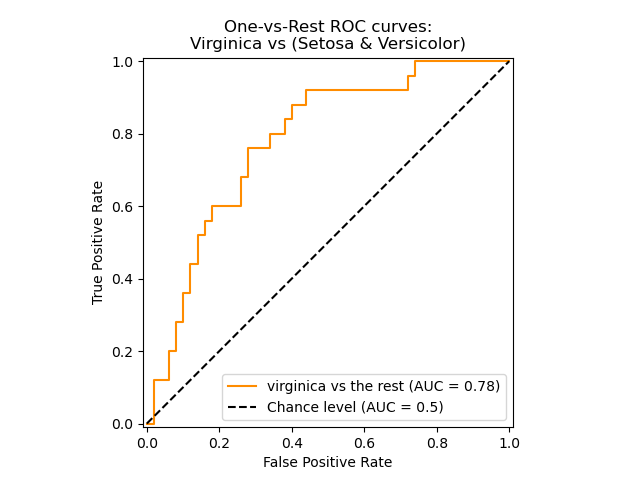
For more information see the Wikipedia article on AUC.
3.3.2.15.1. Binary case
In the binary case, you can either provide the probability estimates, using the classifier.predict_proba() method, or the non-thresholded decision values given by the classifier.decision_function() method. In the case of providing the probability estimates, the probability of the class with the “greater label” should be provided. The “greater label” corresponds to classifier.classes_[1] and thus classifier.predict_proba(X)[:, 1] . Therefore, the y_score parameter is of size (n_samples,).
We can use the probability estimates corresponding to clf.classes_[1] .
Otherwise, we can use the non-thresholded decision values
3.3.2.15.2. Multi-class case
The roc_auc_score function can also be used in multi-class classification. Two averaging strategies are currently supported: the one-vs-one algorithm computes the average of the pairwise ROC AUC scores, and the one-vs-rest algorithm computes the average of the ROC AUC scores for each class against all other classes. In both cases, the predicted labels are provided in an array with values from 0 to n_classes , and the scores correspond to the probability estimates that a sample belongs to a particular class. The OvO and OvR algorithms support weighting uniformly ( average=’macro’ ) and by prevalence ( average=’weighted’ ).
One-vs-one Algorithm: Computes the average AUC of all possible pairwise combinations of classes. [HT2001] defines a multiclass AUC metric weighted uniformly:
where \(c\) is the number of classes and \(\text
(j | k)\) is the AUC with class \(j\) as the positive class and class \(k\) as the negative class. In general, \(\text (j | k) \neq \text (k | j))\) in the multiclass case. This algorithm is used by setting the keyword argument multiclass to ‘ovo’ and average to ‘macro’ . The [HT2001] multiclass AUC metric can be extended to be weighted by the prevalence:
where \(c\) is the number of classes. This algorithm is used by setting the keyword argument multiclass to ‘ovo’ and average to ‘weighted’ . The ‘weighted’ option returns a prevalence-weighted average as described in [FC2009] .
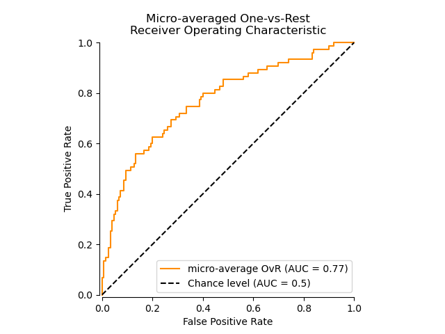
One-vs-rest Algorithm: Computes the AUC of each class against the rest [PD2000] . The algorithm is functionally the same as the multilabel case. To enable this algorithm set the keyword argument multiclass to ‘ovr’ . Additionally to ‘macro’ [F2006] and ‘weighted’ [F2001] averaging, OvR supports ‘micro’ averaging.
In applications where a high false positive rate is not tolerable the parameter max_fpr of roc_auc_score can be used to summarize the ROC curve up to the given limit.
The following figure shows the micro-averaged ROC curve and its corresponding ROC-AUC score for a classifier aimed to distinguish the the different species in the Iris plants dataset :
3.3.2.15.3. Multi-label case
In multi-label classification, the roc_auc_score function is extended by averaging over the labels as above . In this case, you should provide a y_score of shape (n_samples, n_classes) . Thus, when using the probability estimates, one needs to select the probability of the class with the greater label for each output.
And the decision values do not require such processing.
See Multiclass Receiver Operating Characteristic (ROC) for an example of using ROC to evaluate the quality of the output of a classifier.
See Receiver Operating Characteristic (ROC) with cross validation for an example of using ROC to evaluate classifier output quality, using cross-validation.
See Species distribution modeling for an example of using ROC to model species distribution.
Ferri, Cèsar & Hernandez-Orallo, Jose & Modroiu, R. (2009). An Experimental Comparison of Performance Measures for Classification. Pattern Recognition Letters. 30. 27-38.
Provost, F., Domingos, P. (2000). Well-trained PETs: Improving probability estimation trees (Section 6.2), CeDER Working Paper #IS-00-04, Stern School of Business, New York University.
Fawcett, T., 2006. An introduction to ROC analysis. Pattern Recognition Letters, 27(8), pp. 861-874.
Fawcett, T., 2001. Using rule sets to maximize ROC performance In Data Mining, 2001. Proceedings IEEE International Conference, pp. 131-138.
3.3.2.16. Detection error tradeoff (DET)
The function det_curve computes the detection error tradeoff curve (DET) curve [WikipediaDET2017] . Quoting Wikipedia:
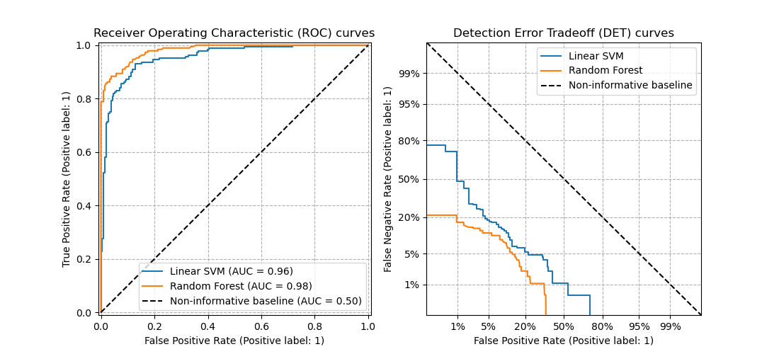
“A detection error tradeoff (DET) graph is a graphical plot of error rates for binary classification systems, plotting false reject rate vs. false accept rate. The x- and y-axes are scaled non-linearly by their standard normal deviates (or just by logarithmic transformation), yielding tradeoff curves that are more linear than ROC curves, and use most of the image area to highlight the differences of importance in the critical operating region.”
DET curves are a variation of receiver operating characteristic (ROC) curves where False Negative Rate is plotted on the y-axis instead of True Positive Rate. DET curves are commonly plotted in normal deviate scale by transformation with \(\phi^<-1>\) (with \(\phi\) being the cumulative distribution function). The resulting performance curves explicitly visualize the tradeoff of error types for given classification algorithms. See [Martin1997] for examples and further motivation.
This figure compares the ROC and DET curves of two example classifiers on the same classification task:
Properties:
DET curves form a linear curve in normal deviate scale if the detection scores are normally (or close-to normally) distributed. It was shown by [Navratil2007] that the reverse is not necessarily true and even more general distributions are able to produce linear DET curves.
The normal deviate scale transformation spreads out the points such that a comparatively larger space of plot is occupied. Therefore curves with similar classification performance might be easier to distinguish on a DET plot.
With False Negative Rate being “inverse” to True Positive Rate the point of perfection for DET curves is the origin (in contrast to the top left corner for ROC curves).
Applications and limitations:
DET curves are intuitive to read and hence allow quick visual assessment of a classifier’s performance. Additionally DET curves can be consulted for threshold analysis and operating point selection. This is particularly helpful if a comparison of error types is required.
On the other hand DET curves do not provide their metric as a single number. Therefore for either automated evaluation or comparison to other classification tasks metrics like the derived area under ROC curve might be better suited.
See Detection error tradeoff (DET) curve for an example comparison between receiver operating characteristic (ROC) curves and Detection error tradeoff (DET) curves.
Wikipedia contributors. Detection error tradeoff. Wikipedia, The Free Encyclopedia. September 4, 2017, 23:33 UTC. Available at: https://en.wikipedia.org/w/index.php?title=Detection_error_tradeoff&oldid=798982054. Accessed February 19, 2018.
A. Martin, G. Doddington, T. Kamm, M. Ordowski, and M. Przybocki, The DET Curve in Assessment of Detection Task Performance, NIST 1997.
J. Navractil and D. Klusacek, “On Linear DETs,” 2007 IEEE International Conference on Acoustics, Speech and Signal Processing — ICASSP ‘07, Honolulu, HI, 2007, pp. IV-229-IV-232.
3.3.2.17. Zero one loss
The zero_one_loss function computes the sum or the average of the 0-1 classification loss ( \(L_<0-1>\) ) over \(n_<\text
>\) . By default, the function normalizes over the sample. To get the sum of the \(L_<0-1>\) , set normalize to False . In multilabel classification, the zero_one_loss scores a subset as one if its labels strictly match the predictions, and as a zero if there are any errors. By default, the function returns the percentage of imperfectly predicted subsets. To get the count of such subsets instead, set normalize to False
If \(\hat
_i\) is the predicted value of the \(i\) -th sample and \(y_i\) is the corresponding true value, then the 0-1 loss \(L_<0-1>\) is defined as: where \(1(x)\) is the indicator function. The zero one loss can also be computed as \(zero-one loss = 1 — accuracy\) .
In the multilabel case with binary label indicators, where the first label set [0,1] has an error:
See Recursive feature elimination with cross-validation for an example of zero one loss usage to perform recursive feature elimination with cross-validation.
3.3.2.18. Brier score loss
The brier_score_loss function computes the Brier score for binary classes [Brier1950] . Quoting Wikipedia:
“The Brier score is a proper score function that measures the accuracy of probabilistic predictions. It is applicable to tasks in which predictions must assign probabilities to a set of mutually exclusive discrete outcomes.”
This function returns the mean squared error of the actual outcome \(y \in \<0,1\>\) and the predicted probability estimate \(p = \operatorname
(y = 1)\) ( predict_proba ) as outputted by: The Brier score loss is also between 0 to 1 and the lower the value (the mean square difference is smaller), the more accurate the prediction is.
Here is a small example of usage of this function:
The Brier score can be used to assess how well a classifier is calibrated. However, a lower Brier score loss does not always mean a better calibration. This is because, by analogy with the bias-variance decomposition of the mean squared error, the Brier score loss can be decomposed as the sum of calibration loss and refinement loss [Bella2012] . Calibration loss is defined as the mean squared deviation from empirical probabilities derived from the slope of ROC segments. Refinement loss can be defined as the expected optimal loss as measured by the area under the optimal cost curve. Refinement loss can change independently from calibration loss, thus a lower Brier score loss does not necessarily mean a better calibrated model. “Only when refinement loss remains the same does a lower Brier score loss always mean better calibration” [Bella2012] , [Flach2008] .
See Probability calibration of classifiers for an example of Brier score loss usage to perform probability calibration of classifiers.
Bella, Ferri, Hernández-Orallo, and Ramírez-Quintana “Calibration of Machine Learning Models” in Khosrow-Pour, M. “Machine learning: concepts, methodologies, tools and applications.” Hershey, PA: Information Science Reference (2012).
Flach, Peter, and Edson Matsubara. “On classification, ranking, and probability estimation.” Dagstuhl Seminar Proceedings. Schloss Dagstuhl-Leibniz-Zentrum fr Informatik (2008).
3.3.2.19. Class likelihood ratios
The class_likelihood_ratios function computes the positive and negative likelihood ratios \(LR_\pm\) for binary classes, which can be interpreted as the ratio of post-test to pre-test odds as explained below. As a consequence, this metric is invariant w.r.t. the class prevalence (the number of samples in the positive class divided by the total number of samples) and can be extrapolated between populations regardless of any possible class imbalance.
The \(LR_\pm\) metrics are therefore very useful in settings where the data available to learn and evaluate a classifier is a study population with nearly balanced classes, such as a case-control study, while the target application, i.e. the general population, has very low prevalence.
The positive likelihood ratio \(LR_+\) is the probability of a classifier to correctly predict that a sample belongs to the positive class divided by the probability of predicting the positive class for a sample belonging to the negative class:
The notation here refers to predicted ( \(P\) ) or true ( \(T\) ) label and the sign \(+\) and \(-\) refer to the positive and negative class, respectively, e.g. \(P+\) stands for “predicted positive”.
Analogously, the negative likelihood ratio \(LR_-\) is the probability of a sample of the positive class being classified as belonging to the negative class divided by the probability of a sample of the negative class being correctly classified:
For classifiers above chance \(LR_+\) above 1 higher is better, while \(LR_-\) ranges from 0 to 1 and lower is better. Values of \(LR_\pm\approx 1\) correspond to chance level.
Notice that probabilities differ from counts, for instance \(\operatorname
(P+|T+)\) is not equal to the number of true positive counts tp (see the wikipedia page for the actual formulas). Interpretation across varying prevalence:
Both class likelihood ratios are interpretable in terms of an odds ratio (pre-test and post-tests):
Odds are in general related to probabilities via
On a given population, the pre-test probability is given by the prevalence. By converting odds to probabilities, the likelihood ratios can be translated into a probability of truly belonging to either class before and after a classifier prediction:
Mathematical divergences:
The positive likelihood ratio is undefined when \(fp = 0\) , which can be interpreted as the classifier perfectly identifying positive cases. If \(fp = 0\) and additionally \(tp = 0\) , this leads to a zero/zero division. This happens, for instance, when using a DummyClassifier that always predicts the negative class and therefore the interpretation as a perfect classifier is lost.
The negative likelihood ratio is undefined when \(tn = 0\) . Such divergence is invalid, as \(LR_- > 1\) would indicate an increase in the odds of a sample belonging to the positive class after being classified as negative, as if the act of classifying caused the positive condition. This includes the case of a DummyClassifier that always predicts the positive class (i.e. when \(tn=fn=0\) ).
Both class likelihood ratios are undefined when \(tp=fn=0\) , which means that no samples of the positive class were present in the testing set. This can also happen when cross-validating highly imbalanced data.
In all the previous cases the class_likelihood_ratios function raises by default an appropriate warning message and returns nan to avoid pollution when averaging over cross-validation folds.
For a worked-out demonstration of the class_likelihood_ratios function, see the example below.
Brenner, H., & Gefeller, O. (1997). Variation of sensitivity, specificity, likelihood ratios and predictive values with disease prevalence. Statistics in medicine, 16(9), 981-991.
3.3.3. Multilabel ranking metrics
In multilabel learning, each sample can have any number of ground truth labels associated with it. The goal is to give high scores and better rank to the ground truth labels.
3.3.3.1. Coverage error
The coverage_error function computes the average number of labels that have to be included in the final prediction such that all true labels are predicted. This is useful if you want to know how many top-scored-labels you have to predict in average without missing any true one. The best value of this metrics is thus the average number of true labels.
Our implementation’s score is 1 greater than the one given in Tsoumakas et al., 2010. This extends it to handle the degenerate case in which an instance has 0 true labels.
Formally, given a binary indicator matrix of the ground truth labels \(y \in \left\<0, 1\right\>^
>\) and the score associated with each label \(\hat \in \mathbb ^ >\) , the coverage is defined as with \(\text
_ = \left|\left\ \geq \hat _ \right\>\right|\) . Given the rank definition, ties in y_scores are broken by giving the maximal rank that would have been assigned to all tied values. Here is a small example of usage of this function:
3.3.3.2. Label ranking average precision
The label_ranking_average_precision_score function implements label ranking average precision (LRAP). This metric is linked to the average_precision_score function, but is based on the notion of label ranking instead of precision and recall.
Label ranking average precision (LRAP) averages over the samples the answer to the following question: for each ground truth label, what fraction of higher-ranked labels were true labels? This performance measure will be higher if you are able to give better rank to the labels associated with each sample. The obtained score is always strictly greater than 0, and the best value is 1. If there is exactly one relevant label per sample, label ranking average precision is equivalent to the mean reciprocal rank.
Formally, given a binary indicator matrix of the ground truth labels \(y \in \left\<0, 1\right\>^
>\) and the score associated with each label \(\hat \in \mathbb ^ >\) , the average precision is defined as where \(\mathcal
_ = \left\ _ \geq \hat _ \right\>\) , \(\text _ = \left|\left\ \geq \hat _ \right\>\right|\) , \(|\cdot|\) computes the cardinality of the set (i.e., the number of elements in the set), and \(||\cdot||_0\) is the \(\ell_0\) “norm” (which computes the number of nonzero elements in a vector). Here is a small example of usage of this function:
3.3.3.3. Ranking loss
The label_ranking_loss function computes the ranking loss which averages over the samples the number of label pairs that are incorrectly ordered, i.e. true labels have a lower score than false labels, weighted by the inverse of the number of ordered pairs of false and true labels. The lowest achievable ranking loss is zero.
Formally, given a binary indicator matrix of the ground truth labels \(y \in \left\<0, 1\right\>^
>\) and the score associated with each label \(\hat \in \mathbb ^ >\) , the ranking loss is defined as where \(|\cdot|\) computes the cardinality of the set (i.e., the number of elements in the set) and \(||\cdot||_0\) is the \(\ell_0\) “norm” (which computes the number of nonzero elements in a vector).
Here is a small example of usage of this function:
Tsoumakas, G., Katakis, I., & Vlahavas, I. (2010). Mining multi-label data. In Data mining and knowledge discovery handbook (pp. 667-685). Springer US.
3.3.3.4. Normalized Discounted Cumulative Gain
Discounted Cumulative Gain (DCG) and Normalized Discounted Cumulative Gain (NDCG) are ranking metrics implemented in dcg_score and ndcg_score ; they compare a predicted order to ground-truth scores, such as the relevance of answers to a query.
From the Wikipedia page for Discounted Cumulative Gain:
“Discounted cumulative gain (DCG) is a measure of ranking quality. In information retrieval, it is often used to measure effectiveness of web search engine algorithms or related applications. Using a graded relevance scale of documents in a search-engine result set, DCG measures the usefulness, or gain, of a document based on its position in the result list. The gain is accumulated from the top of the result list to the bottom, with the gain of each result discounted at lower ranks”
DCG orders the true targets (e.g. relevance of query answers) in the predicted order, then multiplies them by a logarithmic decay and sums the result. The sum can be truncated after the first \(K\) results, in which case we call it DCG@K. NDCG, or NDCG@K is DCG divided by the DCG obtained by a perfect prediction, so that it is always between 0 and 1. Usually, NDCG is preferred to DCG.
Compared with the ranking loss, NDCG can take into account relevance scores, rather than a ground-truth ranking. So if the ground-truth consists only of an ordering, the ranking loss should be preferred; if the ground-truth consists of actual usefulness scores (e.g. 0 for irrelevant, 1 for relevant, 2 for very relevant), NDCG can be used.
For one sample, given the vector of continuous ground-truth values for each target \(y \in \mathbb
^ \) , where \(M\) is the number of outputs, and the prediction \(\hat \) , which induces the ranking function \(f\) , the DCG score is and the NDCG score is the DCG score divided by the DCG score obtained for \(y\) .
Jarvelin, K., & Kekalainen, J. (2002). Cumulated gain-based evaluation of IR techniques. ACM Transactions on Information Systems (TOIS), 20(4), 422-446.
Wang, Y., Wang, L., Li, Y., He, D., Chen, W., & Liu, T. Y. (2013, May). A theoretical analysis of NDCG ranking measures. In Proceedings of the 26th Annual Conference on Learning Theory (COLT 2013)
McSherry, F., & Najork, M. (2008, March). Computing information retrieval performance measures efficiently in the presence of tied scores. In European conference on information retrieval (pp. 414-421). Springer, Berlin, Heidelberg.
3.3.4. Regression metrics
The sklearn.metrics module implements several loss, score, and utility functions to measure regression performance. Some of those have been enhanced to handle the multioutput case: mean_squared_error , mean_absolute_error , r2_score , explained_variance_score , mean_pinball_loss , d2_pinball_score and d2_absolute_error_score .
These functions have a multioutput keyword argument which specifies the way the scores or losses for each individual target should be averaged. The default is ‘uniform_average’ , which specifies a uniformly weighted mean over outputs. If an ndarray of shape (n_outputs,) is passed, then its entries are interpreted as weights and an according weighted average is returned. If multioutput is ‘raw_values’ , then all unaltered individual scores or losses will be returned in an array of shape (n_outputs,) .
The r2_score and explained_variance_score accept an additional value ‘variance_weighted’ for the multioutput parameter. This option leads to a weighting of each individual score by the variance of the corresponding target variable. This setting quantifies the globally captured unscaled variance. If the target variables are of different scale, then this score puts more importance on explaining the higher variance variables. multioutput=’variance_weighted’ is the default value for r2_score for backward compatibility. This will be changed to uniform_average in the future.
3.3.4.1. R² score, the coefficient of determination
The r2_score function computes the coefficient of determination, usually denoted as \(R^2\) .
It represents the proportion of variance (of y) that has been explained by the independent variables in the model. It provides an indication of goodness of fit and therefore a measure of how well unseen samples are likely to be predicted by the model, through the proportion of explained variance.
As such variance is dataset dependent, \(R^2\) may not be meaningfully comparable across different datasets. Best possible score is 1.0 and it can be negative (because the model can be arbitrarily worse). A constant model that always predicts the expected (average) value of y, disregarding the input features, would get an \(R^2\) score of 0.0.
Note: when the prediction residuals have zero mean, the \(R^2\) score and the Explained variance score are identical.
If \(\hat
_i\) is the predicted value of the \(i\) -th sample and \(y_i\) is the corresponding true value for total \(n\) samples, the estimated \(R^2\) is defined as: where \(\bar
= \frac<1> \sum_ y_i\) and \(\sum_ (y_i — \hat _i)^2 = \sum_ \epsilon_i^2\) . Note that r2_score calculates unadjusted \(R^2\) without correcting for bias in sample variance of y.
In the particular case where the true target is constant, the \(R^2\) score is not finite: it is either NaN (perfect predictions) or -Inf (imperfect predictions). Such non-finite scores may prevent correct model optimization such as grid-search cross-validation to be performed correctly. For this reason the default behaviour of r2_score is to replace them with 1.0 (perfect predictions) or 0.0 (imperfect predictions). If force_finite is set to False , this score falls back on the original \(R^2\) definition.
Here is a small example of usage of the r2_score function:
See Lasso and Elastic Net for Sparse Signals for an example of R² score usage to evaluate Lasso and Elastic Net on sparse signals.
3.3.4.2. Mean absolute error
The mean_absolute_error function computes mean absolute error, a risk metric corresponding to the expected value of the absolute error loss or \(l1\) -norm loss.
If \(\hat
_i\) is the predicted value of the \(i\) -th sample, and \(y_i\) is the corresponding true value, then the mean absolute error (MAE) estimated over \(n_<\text >\) is defined as Here is a small example of usage of the mean_absolute_error function:
3.3.4.3. Mean squared error
The mean_squared_error function computes mean square error, a risk metric corresponding to the expected value of the squared (quadratic) error or loss.
If \(\hat
_i\) is the predicted value of the \(i\) -th sample, and \(y_i\) is the corresponding true value, then the mean squared error (MSE) estimated over \(n_<\text >\) is defined as Here is a small example of usage of the mean_squared_error function:
See Gradient Boosting regression for an example of mean squared error usage to evaluate gradient boosting regression.
3.3.4.4. Mean squared logarithmic error
The mean_squared_log_error function computes a risk metric corresponding to the expected value of the squared logarithmic (quadratic) error or loss.
If \(\hat
_i\) is the predicted value of the \(i\) -th sample, and \(y_i\) is the corresponding true value, then the mean squared logarithmic error (MSLE) estimated over \(n_<\text >\) is defined as Where \(\log_e (x)\) means the natural logarithm of \(x\) . This metric is best to use when targets having exponential growth, such as population counts, average sales of a commodity over a span of years etc. Note that this metric penalizes an under-predicted estimate greater than an over-predicted estimate.
Here is a small example of usage of the mean_squared_log_error function:
3.3.4.5. Mean absolute percentage error
The mean_absolute_percentage_error (MAPE), also known as mean absolute percentage deviation (MAPD), is an evaluation metric for regression problems. The idea of this metric is to be sensitive to relative errors. It is for example not changed by a global scaling of the target variable.
If \(\hat
_i\) is the predicted value of the \(i\) -th sample and \(y_i\) is the corresponding true value, then the mean absolute percentage error (MAPE) estimated over \(n_<\text >\) is defined as where \(\epsilon\) is an arbitrary small yet strictly positive number to avoid undefined results when y is zero.
The mean_absolute_percentage_error function supports multioutput.
Here is a small example of usage of the mean_absolute_percentage_error function:
In above example, if we had used mean_absolute_error , it would have ignored the small magnitude values and only reflected the error in prediction of highest magnitude value. But that problem is resolved in case of MAPE because it calculates relative percentage error with respect to actual output.
3.3.4.6. Median absolute error
The median_absolute_error is particularly interesting because it is robust to outliers. The loss is calculated by taking the median of all absolute differences between the target and the prediction.
If \(\hat
_i\) is the predicted value of the \(i\) -th sample and \(y_i\) is the corresponding true value, then the median absolute error (MedAE) estimated over \(n_<\text >\) is defined as The median_absolute_error does not support multioutput.
Here is a small example of usage of the median_absolute_error function:
3.3.4.7. Max error
The max_error function computes the maximum residual error , a metric that captures the worst case error between the predicted value and the true value. In a perfectly fitted single output regression model, max_error would be 0 on the training set and though this would be highly unlikely in the real world, this metric shows the extent of error that the model had when it was fitted.
If \(\hat
_i\) is the predicted value of the \(i\) -th sample, and \(y_i\) is the corresponding true value, then the max error is defined as Here is a small example of usage of the max_error function:
The max_error does not support multioutput.
3.3.4.8. Explained variance score
If \(\hat
\) is the estimated target output, \(y\) the corresponding (correct) target output, and \(Var\) is Variance, the square of the standard deviation, then the explained variance is estimated as follow: The best possible score is 1.0, lower values are worse.
The difference between the explained variance score and the R² score, the coefficient of determination is that when the explained variance score does not account for systematic offset in the prediction. For this reason, the R² score, the coefficient of determination should be preferred in general.
In the particular case where the true target is constant, the Explained Variance score is not finite: it is either NaN (perfect predictions) or -Inf (imperfect predictions). Such non-finite scores may prevent correct model optimization such as grid-search cross-validation to be performed correctly. For this reason the default behaviour of explained_variance_score is to replace them with 1.0 (perfect predictions) or 0.0 (imperfect predictions). You can set the force_finite parameter to False to prevent this fix from happening and fallback on the original Explained Variance score.
Here is a small example of usage of the explained_variance_score function:
3.3.4.9. Mean Poisson, Gamma, and Tweedie deviances
The mean_tweedie_deviance function computes the mean Tweedie deviance error with a power parameter ( \(p\) ). This is a metric that elicits predicted expectation values of regression targets.
Following special cases exist,
when power=0 it is equivalent to mean_squared_error .
when power=1 it is equivalent to mean_poisson_deviance .
when power=2 it is equivalent to mean_gamma_deviance .
If \(\hat
_i\) is the predicted value of the \(i\) -th sample, and \(y_i\) is the corresponding true value, then the mean Tweedie deviance error (D) for power \(p\) , estimated over \(n_<\text >\) is defined as Tweedie deviance is a homogeneous function of degree 2-power . Thus, Gamma distribution with power=2 means that simultaneously scaling y_true and y_pred has no effect on the deviance. For Poisson distribution power=1 the deviance scales linearly, and for Normal distribution ( power=0 ), quadratically. In general, the higher power the less weight is given to extreme deviations between true and predicted targets.
For instance, let’s compare the two predictions 1.5 and 150 that are both 50% larger than their corresponding true value.
The mean squared error ( power=0 ) is very sensitive to the prediction difference of the second point,:
If we increase power to 1,:
the difference in errors decreases. Finally, by setting, power=2 :
we would get identical errors. The deviance when power=2 is thus only sensitive to relative errors.
3.3.4.10. Pinball loss
The mean_pinball_loss function is used to evaluate the predictive performance of quantile regression models.
The value of pinball loss is equivalent to half of mean_absolute_error when the quantile parameter alpha is set to 0.5.
Here is a small example of usage of the mean_pinball_loss function:
It is possible to build a scorer object with a specific choice of alpha :
Such a scorer can be used to evaluate the generalization performance of a quantile regressor via cross-validation:
It is also possible to build scorer objects for hyper-parameter tuning. The sign of the loss must be switched to ensure that greater means better as explained in the example linked below.
See Prediction Intervals for Gradient Boosting Regression for an example of using the pinball loss to evaluate and tune the hyper-parameters of quantile regression models on data with non-symmetric noise and outliers.
3.3.4.11. D² score
The D² score computes the fraction of deviance explained. It is a generalization of R², where the squared error is generalized and replaced by a deviance of choice \(\text
(y, \hat )\) (e.g., Tweedie, pinball or mean absolute error). D² is a form of a skill score. It is calculated as Where \(y_<\text
>\) is the optimal prediction of an intercept-only model (e.g., the mean of y_true for the Tweedie case, the median for absolute error and the alpha-quantile for pinball loss). Like R², the best possible score is 1.0 and it can be negative (because the model can be arbitrarily worse). A constant model that always predicts \(y_<\text
>\) , disregarding the input features, would get a D² score of 0.0. 3.3.4.11.1. D² Tweedie score
The d2_tweedie_score function implements the special case of D² where \(\text
(y, \hat )\) is the Tweedie deviance, see Mean Poisson, Gamma, and Tweedie deviances . It is also known as D² Tweedie and is related to McFadden’s likelihood ratio index. The argument power defines the Tweedie power as for mean_tweedie_deviance . Note that for power=0 , d2_tweedie_score equals r2_score (for single targets).
A scorer object with a specific choice of power can be built by:
3.3.4.11.2. D² pinball score
The d2_pinball_score function implements the special case of D² with the pinball loss, see Pinball loss , i.e.:
The argument alpha defines the slope of the pinball loss as for mean_pinball_loss ( Pinball loss ). It determines the quantile level alpha for which the pinball loss and also D² are optimal. Note that for alpha=0.5 (the default) d2_pinball_score equals d2_absolute_error_score .
A scorer object with a specific choice of alpha can be built by:
3.3.4.11.3. D² absolute error score
The d2_absolute_error_score function implements the special case of the Mean absolute error :
Here are some usage examples of the d2_absolute_error_score function:
3.3.4.12. Visual evaluation of regression models
Among methods to assess the quality of regression models, scikit-learn provides the PredictionErrorDisplay class. It allows to visually inspect the prediction errors of a model in two different manners.
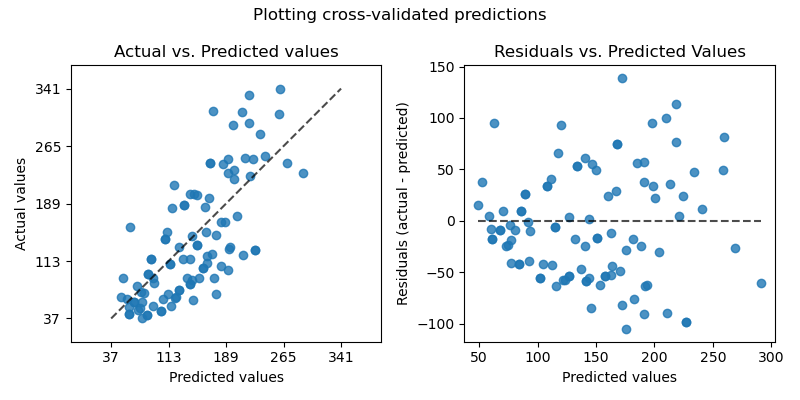
The plot on the left shows the actual values vs predicted values. For a noise-free regression task aiming to predict the (conditional) expectation of y , a perfect regression model would display data points on the diagonal defined by predicted equal to actual values. The further away from this optimal line, the larger the error of the model. In a more realistic setting with irreducible noise, that is, when not all the variations of y can be explained by features in X , then the best model would lead to a cloud of points densely arranged around the diagonal.
Note that the above only holds when the predicted values is the expected value of y given X . This is typically the case for regression models that minimize the mean squared error objective function or more generally the mean Tweedie deviance for any value of its “power” parameter.
When plotting the predictions of an estimator that predicts a quantile of y given X , e.g. QuantileRegressor or any other model minimizing the pinball loss , a fraction of the points are either expected to lie above or below the diagonal depending on the estimated quantile level.
All in all, while intuitive to read, this plot does not really inform us on what to do to obtain a better model.
The right-hand side plot shows the residuals (i.e. the difference between the actual and the predicted values) vs. the predicted values.
This plot makes it easier to visualize if the residuals follow and homoscedastic or heteroschedastic distribution.
In particular, if the true distribution of y|X is Poisson or Gamma distributed, it is expected that the variance of the residuals of the optimal model would grow with the predicted value of E[y|X] (either linearly for Poisson or quadratically for Gamma).
When fitting a linear least squares regression model (see LinearRegression and Ridge ), we can use this plot to check if some of the model assumptions are met, in particular that the residuals should be uncorrelated, their expected value should be null and that their variance should be constant (homoschedasticity).
If this is not the case, and in particular if the residuals plot show some banana-shaped structure, this is a hint that the model is likely mis-specified and that non-linear feature engineering or switching to a non-linear regression model might be useful.
Refer to the example below to see a model evaluation that makes use of this display.
See Effect of transforming the targets in regression model for an example on how to use PredictionErrorDisplay to visualize the prediction quality improvement of a regression model obtained by transforming the target before learning.
3.3.5. Clustering metrics
The sklearn.metrics module implements several loss, score, and utility functions. For more information see the Clustering performance evaluation section for instance clustering, and Biclustering evaluation for biclustering.
3.3.6. Dummy estimators
When doing supervised learning, a simple sanity check consists of comparing one’s estimator against simple rules of thumb. DummyClassifier implements several such simple strategies for classification:
stratified generates random predictions by respecting the training set class distribution.
most_frequent always predicts the most frequent label in the training set.
prior always predicts the class that maximizes the class prior (like most_frequent ) and predict_proba returns the class prior.
uniform generates predictions uniformly at random.
A major motivation of this method is F1-scoring, when the positive class is in the minority.
Note that with all these strategies, the predict method completely ignores the input data!
To illustrate DummyClassifier , first let’s create an imbalanced dataset:
Next, let’s compare the accuracy of SVC and most_frequent :
We see that SVC doesn’t do much better than a dummy classifier. Now, let’s change the kernel:
We see that the accuracy was boosted to almost 100%. A cross validation strategy is recommended for a better estimate of the accuracy, if it is not too CPU costly. For more information see the Cross-validation: evaluating estimator performance section. Moreover if you want to optimize over the parameter space, it is highly recommended to use an appropriate methodology; see the Tuning the hyper-parameters of an estimator section for details.
More generally, when the accuracy of a classifier is too close to random, it probably means that something went wrong: features are not helpful, a hyperparameter is not correctly tuned, the classifier is suffering from class imbalance, etc…
DummyRegressor also implements four simple rules of thumb for regression:
mean always predicts the mean of the training targets.
median always predicts the median of the training targets.
quantile always predicts a user provided quantile of the training targets.
constant always predicts a constant value that is provided by the user.
In all these strategies, the predict method completely ignores the input data.
Регрессионный анализ в DataScience. Простая линейная регрессия. Библиотека statsmodels
Про регрессионный анализ вообще, и его применение в DataScience написано очень много. Есть множество учебников, монографий, справочников и статей по прикладной статистике, огромное количество информации в интернете, примеров расчетов. Можно найти множество кейсов, реализованных с использованием средств Python. Казалось бы — что тут еще можно добавить?
Однако, как всегда, есть нюансы:
1. Регрессионный анализ — это прежде всего процесс, набор действий исследователя по определенному алгоритму: «подготовка исходных данных — построение модели — анализ модели — прогнозирование с помощью модели». Это ключевая особенность. Не представляет особой сложности сформировать DataFrame исходных данных и построить модель, запустить процедуру из библиотеки statsmodels. Однако подготовка исходных данных и последующий анализ модели требуют гораздо больших затрат человеко-часов специалиста и строк программного кода, чем, собственно, построение модели. На этих этапах часто приходится возвращаться назад, корректировать модель или исходные данные. Этому, к сожалению, во многих источниках, не удаляется достойного внимания, а иногда — и совсем не уделяется внимания, что приводит к превратному представлению о регрессионном анализе.
2. Далеко не во всех источниках уделяется должное внимание интерпретации промежуточных и финальных результатов. Специалист должен уметь интерпретировать каждую цифру, полученную в ходе работы над моделью.
3. Далеко не все процедуры на этапах подготовки исходных данных или анализа модели в источниках разобраны подробно. Например, про проверку значимости коэффициента детерминации найти информацию не представляет труда, а вот про проверку адекватности модели, построение доверительных интервалов регрессии или про специфические процедуры (например, тест Уайта на гетероскедастичность) информации гораздо меньше.
4. Своеобразная сложность может возникнуть с проверкой статистических гипотез: для отечественной литературы по прикладной статистике больше характерно проверять гипотезы путем сравнения расчетного значения критерия с табличным, а в иностранных источниках чаще определяется расчетный уровень значимости и сравнивается с заданным (чаще всего 0.05 = 1-0.95). В разных источниках информации реализованы разные подходы. Инструменты python (прежде всего библиотеки scipy и statsmodels) также в основном оперируют с расчетным уровнем значимости.
5. Ну и, наконец, нельзя не отметить, что техническая документация библиотеки statsmodels составлена, на мой взгляд, далеко не идеально: информация излагается путано, изобилует повторами и пропусками, описание классов, функций и свойств выполнено фрагментарно и количество примеров расчетов — явно недостаточно.
Поэтому я решил написать ряд обзоров по регрессионному анализу средствами Python, в которых акцент будет сделан на практических примерах, алгоритме действий исследователя, интерпретации всех полученных результатов, конкретных методических рекомендациях. Буду стараться по возможности избегать теории (хотя совсем без нее получится) — все-таки предполагается, что специалист DataScience должен знать теорию вероятностей и математическую статистику, хотя бы в рамках курса высшей математики для технического или экономического вуза.
В данном статье остановимся на самои простом, классическом, стереотипном случае — простой линейной регрессии (simple linear regression), или как ее еще принято называть — парной линейной регрессионной модели (ПЛРМ) — в ситуации, когда исследователя не подстерегают никакие подводные камни и каверзы — исходные данные подчиняются нормальному закону, в выборке отсутствуют аномальные значения, отсутствует ложная корреляция. Более сложные случаи рассмотрим в дальнейшем.
Для построение регрессионной модели будем пользоваться библиотекой statsmodels.
В данной статье мы рассмотрим по возможности полный набор статистических процедур. Некоторые из них (например, дескриптивная статистика или дисперсионный анализ регрессионной модели) могут показаться избыточными. Все так, но эти процедуры улучшают наше представление о процессе и об исходных данных, поэтому в разбор я их включил, а каждый исследователь сам вправе для себя определить, потребуются ему эти процедуры или нет.
Краткий обзор источников
Источников информации по корреляционному и регрессионному анализу огромное количество, в них можно просто утонуть. Поэтому позволю себе просто порекомендовать ряд источников, на мой взгляд, наиболее полезных:
Кобзарь А.И. Прикладная математическая статистика. Для инженеров и научных работников. — М.: ФИЗМАТЛИТ, 2006. — 816 с.
Львовский Е.Н. Статистические методы построения эмпирических формул. — М.: Высшая школа, 1988. — 239 с.
Фёрстер Э., Рёнц Б. Методы корреляционного и регрессионного анализа / пер с нем. — М.: Финансы и статистика, 1983. — 302 с.
Афифи А., Эйзен С. Статистический анализ. Подход с использованием ЭВМ / пер с англ. — М.: Мир, 1982. — 488 с.
Дрейпер Н., Смит Г. Прикладной регрессионный анализ. Книга 1 / пер.с англ. — М.: Финансы и статистика, 1986. — 366 с.
Айвазян С.А. и др. Прикладная статистика: Исследование зависимостей. — М.: Финансы и статистика, 1985. — 487 с.
Прикладная статистика. Основы эконометрики: В 2 т. 2-е изд., испр. — Т.2: Айвазян С.А. Основы эконометрики. — М.: ЮНИТИ-ДАНА, 2001. — 432 с.
Магнус Я.Р. и др. Эконометрика. Начальный курс — М.: Дело, 2004. — 576 с.
Носко В.П. Эконометрика. Книга 1. — М.: Издательский дом «Дело» РАНХиГС, 2011. — 672 с.
Брюс П. Практическая статистика для специалистов Data Science / пер. с англ. — СПб.: БХВ-Петербург, 2018. — 304 с.
Уатт Дж. и др. Машинное обучение: основы, алгоритмы и практика применения / пер. с англ. — СПб.: БХВ-Петербург, 2022. — 640 с.
Прежде всего следует упомянуть справочник Кобзаря А.И. [1] — это безусловно выдающийся труд. Ничего подобного даже близко не издавалось. Всем рекомендую иметь под рукой.
Есть очень хорошее практическое пособие [2] — для начинающих и практиков.>
Добротная работа немецких авторов [3]. Все разобрано подробно, обстоятельно, с примерами — очень хорошая книга. Примеры приведены из области экономики.
Еще одна добротная работа — [4], с примерами медико-биологического характера.
Работа [5] считается одним из наиболее полных изложений прикладного регрессионного анализа.
Более сложные работы — [6] (классика жанра), [7], [8], [9] — выдержаны на достаточно высоком математическом уровне, примеры из экономической области.
Свежие работы [10] (с примерами на языке R) и [11] (с примерами на python).
Cтатьи
Статей про регрессионный анализ в DataScience очень много, обращаю внимание на некоторые весьма полезные из них.
Серия статей «Python, корреляция и регрессия», охватывающая весь процесс регрессионного анализа: