Как построить распределение в python

Visualizing distributions of data#

An early step in any effort to analyze or model data should be to understand how the variables are distributed. Techniques for distribution visualization can provide quick answers to many important questions. What range do the observations cover? What is their central tendency? Are they heavily skewed in one direction? Is there evidence for bimodality? Are there significant outliers? Do the answers to these questions vary across subsets defined by other variables?

The distributions module contains several functions designed to answer questions such as these. The axes-level functions are histplot() , kdeplot() , ecdfplot() , and rugplot() . They are grouped together within the figure-level displot() , jointplot() , and pairplot() functions.

There are several different approaches to visualizing a distribution, and each has its relative advantages and drawbacks. It is important to understand these factors so that you can choose the best approach for your particular aim.

Plotting univariate histograms#

Perhaps the most common approach to visualizing a distribution is the histogram. This is the default approach in displot() , which uses the same underlying code as histplot() . A histogram is a bar plot where the axis representing the data variable is divided into a set of discrete bins and the count of observations falling within each bin is shown using the height of the corresponding bar:

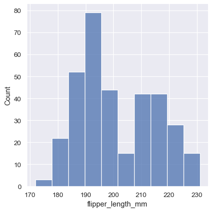
This plot immediately affords a few insights about the flipper_length_mm variable. For instance, we can see that the most common flipper length is about 195 mm, but the distribution appears bimodal, so this one number does not represent the data well.

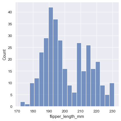
Choosing the bin size#

The size of the bins is an important parameter, and using the wrong bin size can mislead by obscuring important features of the data or by creating apparent features out of random variability. By default, displot() / histplot() choose a default bin size based on the variance of the data and the number of observations. But you should not be over-reliant on such automatic approaches, because they depend on particular assumptions about the structure of your data. It is always advisable to check that your impressions of the distribution are consistent across different bin sizes. To choose the size directly, set the binwidth parameter:

In other circumstances, it may make more sense to specify the number of bins, rather than their size:

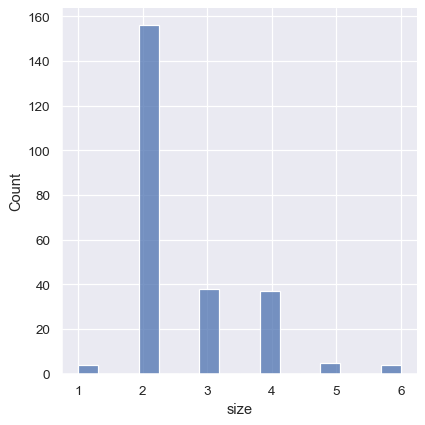
One example of a situation where defaults fail is when the variable takes a relatively small number of integer values. In that case, the default bin width may be too small, creating awkward gaps in the distribution:

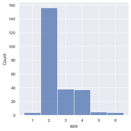
One approach would be to specify the precise bin breaks by passing an array to bins :

This can also be accomplished by setting discrete=True , which chooses bin breaks that represent the unique values in a dataset with bars that are centered on their corresponding value.

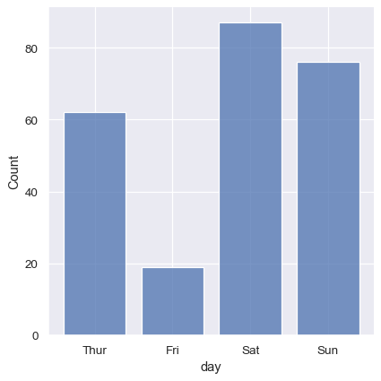
It’s also possible to visualize the distribution of a categorical variable using the logic of a histogram. Discrete bins are automatically set for categorical variables, but it may also be helpful to “shrink” the bars slightly to emphasize the categorical nature of the axis:

Conditioning on other variables#

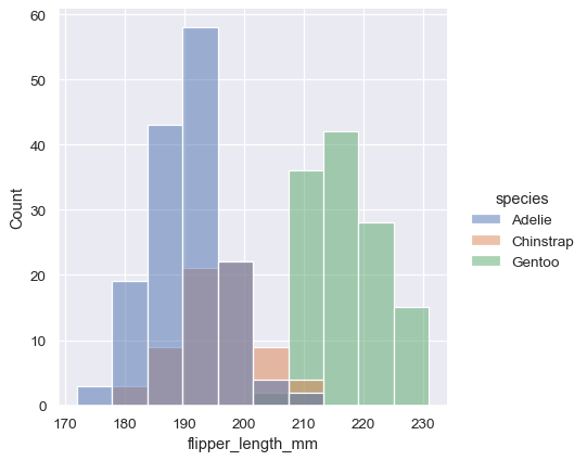
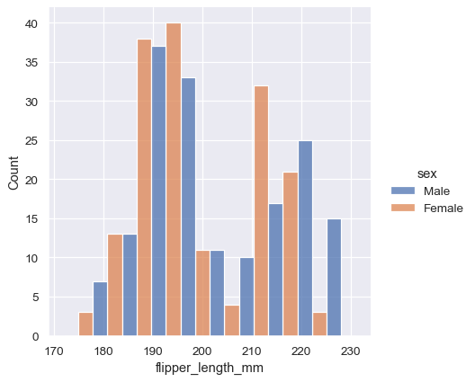
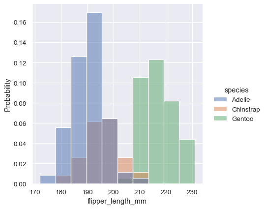
Once you understand the distribution of a variable, the next step is often to ask whether features of that distribution differ across other variables in the dataset. For example, what accounts for the bimodal distribution of flipper lengths that we saw above? displot() and histplot() provide support for conditional subsetting via the hue semantic. Assigning a variable to hue will draw a separate histogram for each of its unique values and distinguish them by color:

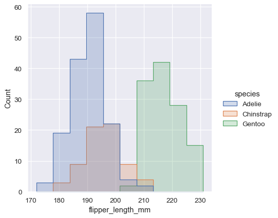
By default, the different histograms are “layered” on top of each other and, in some cases, they may be difficult to distinguish. One option is to change the visual representation of the histogram from a bar plot to a “step” plot:

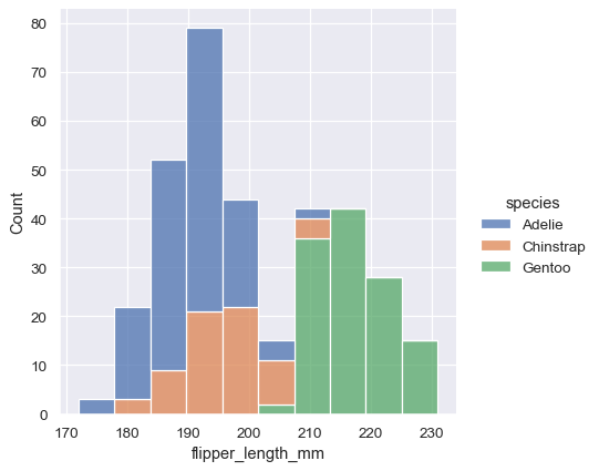
Alternatively, instead of layering each bar, they can be “stacked”, or moved vertically. In this plot, the outline of the full histogram will match the plot with only a single variable:

The stacked histogram emphasizes the part-whole relationship between the variables, but it can obscure other features (for example, it is difficult to determine the mode of the Adelie distribution. Another option is “dodge” the bars, which moves them horizontally and reduces their width. This ensures that there are no overlaps and that the bars remain comparable in terms of height. But it only works well when the categorical variable has a small number of levels:

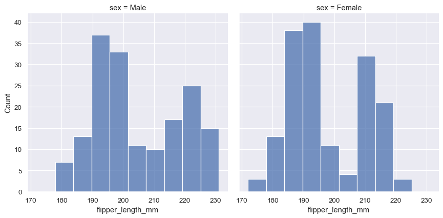
Because displot() is a figure-level function and is drawn onto a FacetGrid , it is also possible to draw each individual distribution in a separate subplot by assigning the second variable to col or row rather than (or in addition to) hue . This represents the distribution of each subset well, but it makes it more difficult to draw direct comparisons:

None of these approaches are perfect, and we will soon see some alternatives to a histogram that are better-suited to the task of comparison.

Normalized histogram statistics#

Before we do, another point to note is that, when the subsets have unequal numbers of observations, comparing their distributions in terms of counts may not be ideal. One solution is to normalize the counts using the stat parameter:

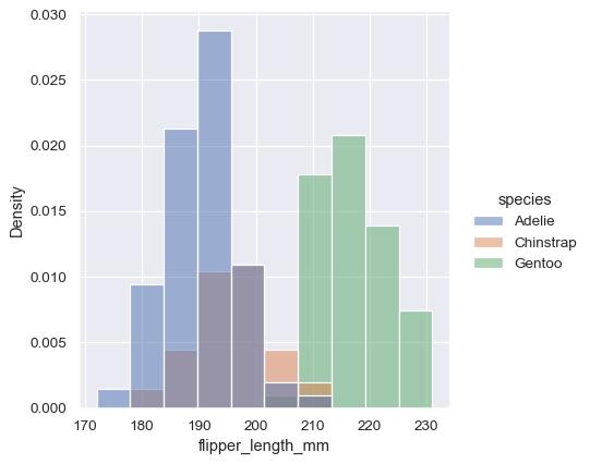
By default, however, the normalization is applied to the entire distribution, so this simply rescales the height of the bars. By setting common_norm=False , each subset will be normalized independently:

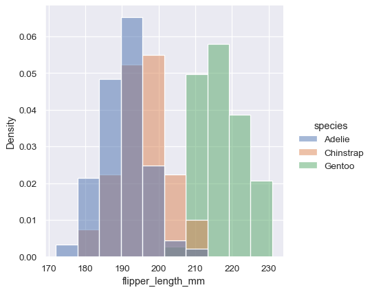
Density normalization scales the bars so that their areas sum to 1. As a result, the density axis is not directly interpretable. Another option is to normalize the bars to that their heights sum to 1. This makes most sense when the variable is discrete, but it is an option for all histograms:

Kernel density estimation#

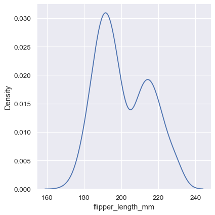
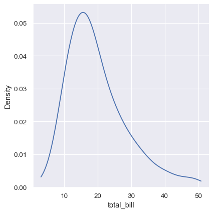
A histogram aims to approximate the underlying probability density function that generated the data by binning and counting observations. Kernel density estimation (KDE) presents a different solution to the same problem. Rather than using discrete bins, a KDE plot smooths the observations with a Gaussian kernel, producing a continuous density estimate:

Choosing the smoothing bandwidth#

Much like with the bin size in the histogram, the ability of the KDE to accurately represent the data depends on the choice of smoothing bandwidth. An over-smoothed estimate might erase meaningful features, but an under-smoothed estimate can obscure the true shape within random noise. The easiest way to check the robustness of the estimate is to adjust the default bandwidth:

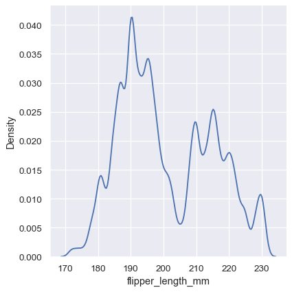
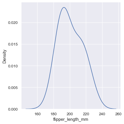
Note how the narrow bandwidth makes the bimodality much more apparent, but the curve is much less smooth. In contrast, a larger bandwidth obscures the bimodality almost completely:

Conditioning on other variables#

As with histograms, if you assign a hue variable, a separate density estimate will be computed for each level of that variable:

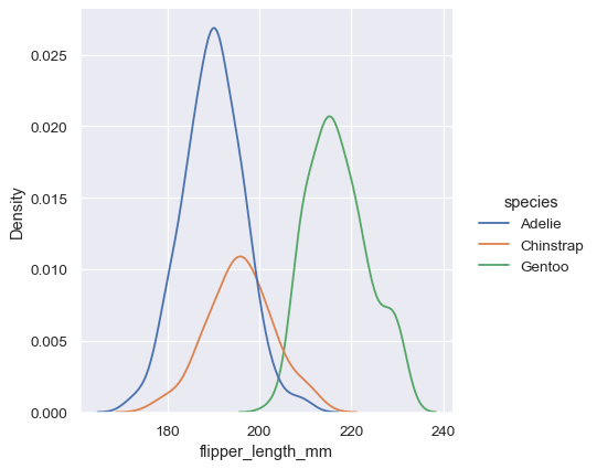
In many cases, the layered KDE is easier to interpret than the layered histogram, so it is often a good choice for the task of comparison. Many of the same options for resolving multiple distributions apply to the KDE as well, however:

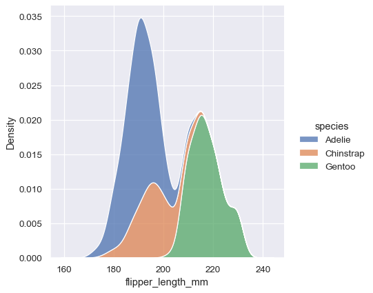
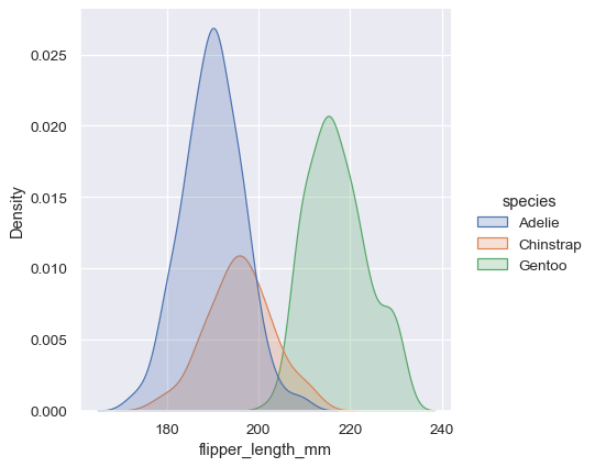
Note how the stacked plot filled in the area between each curve by default. It is also possible to fill in the curves for single or layered densities, although the default alpha value (opacity) will be different, so that the individual densities are easier to resolve.

Kernel density estimation pitfalls#

KDE plots have many advantages. Important features of the data are easy to discern (central tendency, bimodality, skew), and they afford easy comparisons between subsets. But there are also situations where KDE poorly represents the underlying data. This is because the logic of KDE assumes that the underlying distribution is smooth and unbounded. One way this assumption can fail is when a variable reflects a quantity that is naturally bounded. If there are observations lying close to the bound (for example, small values of a variable that cannot be negative), the KDE curve may extend to unrealistic values:

This can be partially avoided with the cut parameter, which specifies how far the curve should extend beyond the extreme datapoints. But this influences only where the curve is drawn; the density estimate will still smooth over the range where no data can exist, causing it to be artificially low at the extremes of the distribution:

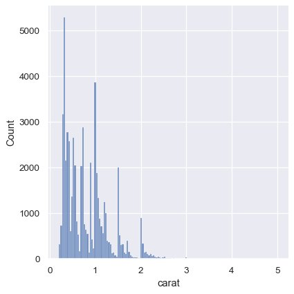
The KDE approach also fails for discrete data or when data are naturally continuous but specific values are over-represented. The important thing to keep in mind is that the KDE will always show you a smooth curve, even when the data themselves are not smooth. For example, consider this distribution of diamond weights:

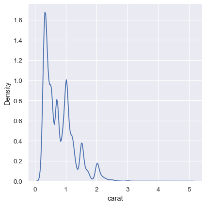
While the KDE suggests that there are peaks around specific values, the histogram reveals a much more jagged distribution:

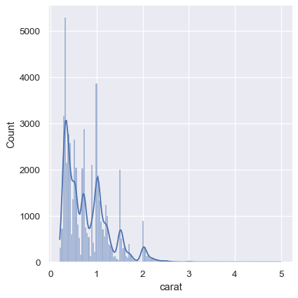
As a compromise, it is possible to combine these two approaches. While in histogram mode, displot() (as with histplot() ) has the option of including the smoothed KDE curve (note kde=True , not kind="kde" ):

Empirical cumulative distributions#

A third option for visualizing distributions computes the “empirical cumulative distribution function” (ECDF). This plot draws a monotonically-increasing curve through each datapoint such that the height of the curve reflects the proportion of observations with a smaller value:

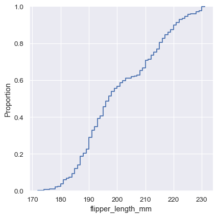
The ECDF plot has two key advantages. Unlike the histogram or KDE, it directly represents each datapoint. That means there is no bin size or smoothing parameter to consider. Additionally, because the curve is monotonically increasing, it is well-suited for comparing multiple distributions:

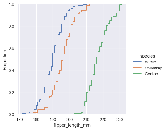
The major downside to the ECDF plot is that it represents the shape of the distribution less intuitively than a histogram or density curve. Consider how the bimodality of flipper lengths is immediately apparent in the histogram, but to see it in the ECDF plot, you must look for varying slopes. Nevertheless, with practice, you can learn to answer all of the important questions about a distribution by examining the ECDF, and doing so can be a powerful approach.

Visualizing bivariate distributions#

All of the examples so far have considered univariate distributions: distributions of a single variable, perhaps conditional on a second variable assigned to hue . Assigning a second variable to y , however, will plot a bivariate distribution:

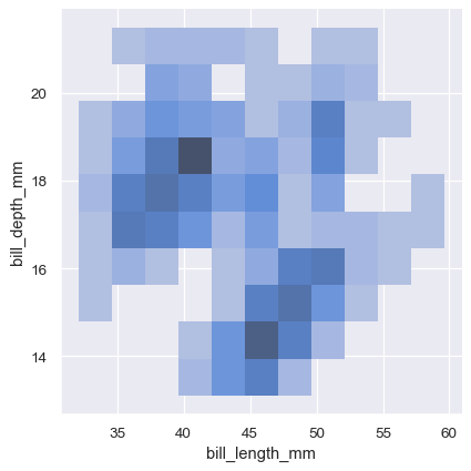
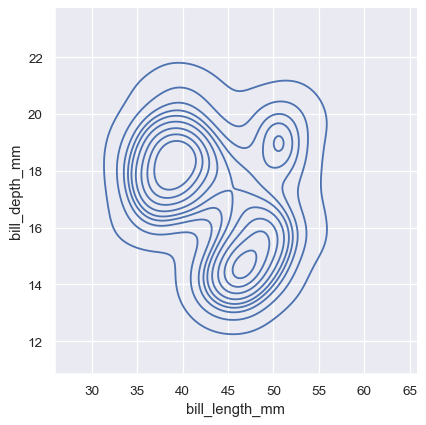
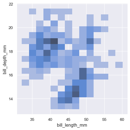
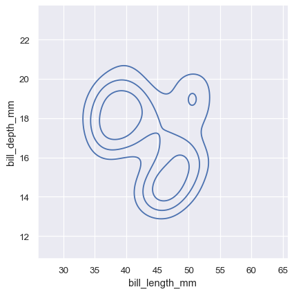
A bivariate histogram bins the data within rectangles that tile the plot and then shows the count of observations within each rectangle with the fill color (analogous to a heatmap() ). Similarly, a bivariate KDE plot smoothes the (x, y) observations with a 2D Gaussian. The default representation then shows the contours of the 2D density:

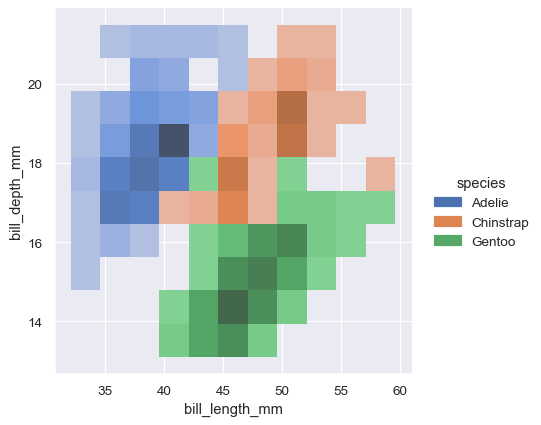
Assigning a hue variable will plot multiple heatmaps or contour sets using different colors. For bivariate histograms, this will only work well if there is minimal overlap between the conditional distributions:

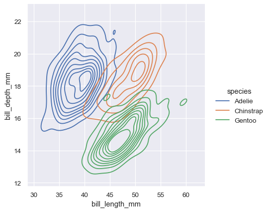
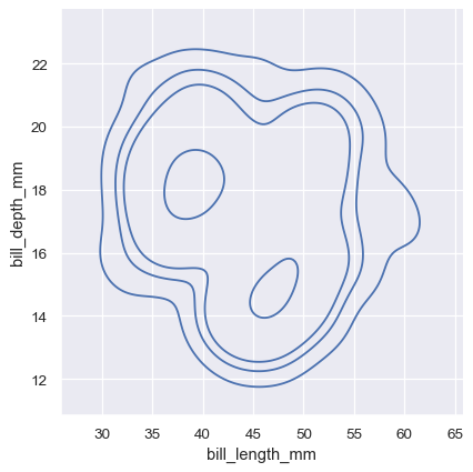
The contour approach of the bivariate KDE plot lends itself better to evaluating overlap, although a plot with too many contours can get busy:

Just as with univariate plots, the choice of bin size or smoothing bandwidth will determine how well the plot represents the underlying bivariate distribution. The same parameters apply, but they can be tuned for each variable by passing a pair of values:

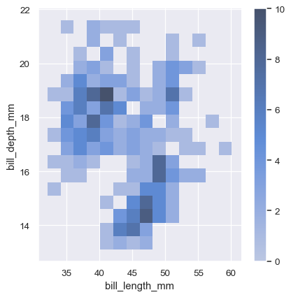
To aid interpretation of the heatmap, add a colorbar to show the mapping between counts and color intensity:

The meaning of the bivariate density contours is less straightforward. Because the density is not directly interpretable, the contours are drawn at iso-proportions of the density, meaning that each curve shows a level set such that some proportion p of the density lies below it. The p values are evenly spaced, with the lowest level contolled by the thresh parameter and the number controlled by levels :

The levels parameter also accepts a list of values, for more control:

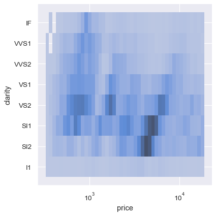
The bivariate histogram allows one or both variables to be discrete. Plotting one discrete and one continuous variable offers another way to compare conditional univariate distributions:

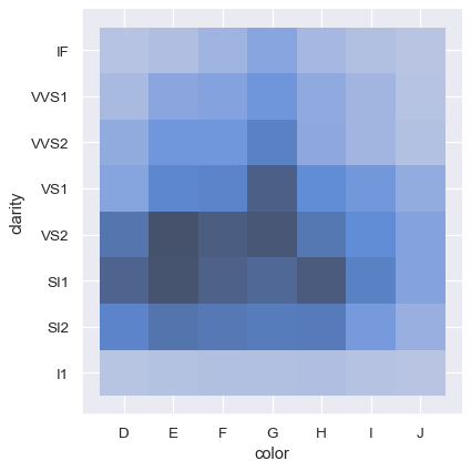
In contrast, plotting two discrete variables is an easy to way show the cross-tabulation of the observations:

Distribution visualization in other settings#

Several other figure-level plotting functions in seaborn make use of the histplot() and kdeplot() functions.

Plotting joint and marginal distributions#

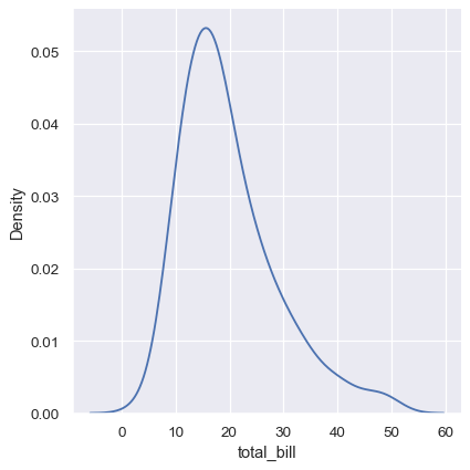
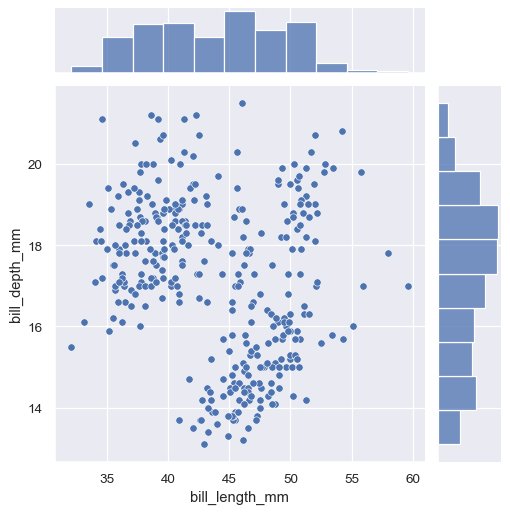
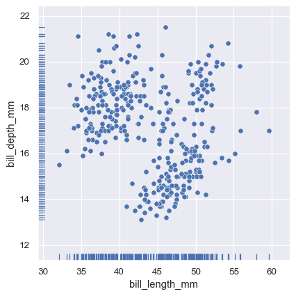
The first is jointplot() , which augments a bivariate relatonal or distribution plot with the marginal distributions of the two variables. By default, jointplot() represents the bivariate distribution using scatterplot() and the marginal distributions using histplot() :

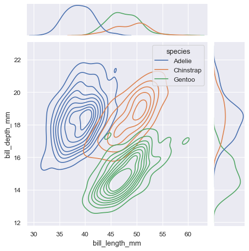
Similar to displot() , setting a different kind="kde" in jointplot() will change both the joint and marginal plots the use kdeplot() :

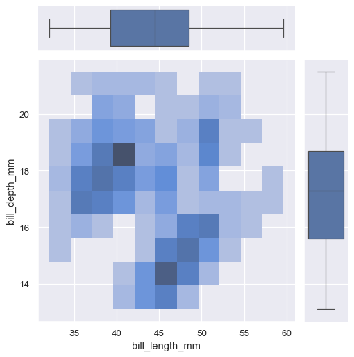
jointplot() is a convenient interface to the JointGrid class, which offeres more flexibility when used directly:

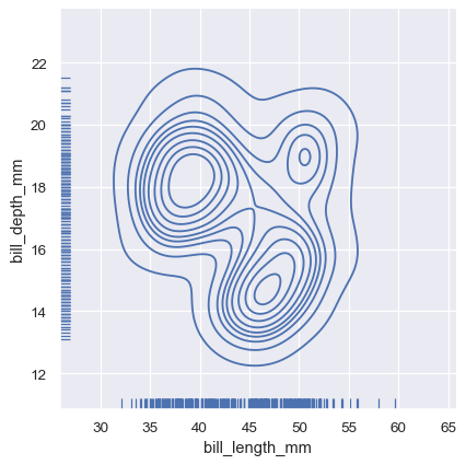
A less-obtrusive way to show marginal distributions uses a “rug” plot, which adds a small tick on the edge of the plot to represent each individual observation. This is built into displot() :

And the axes-level rugplot() function can be used to add rugs on the side of any other kind of plot:

Plotting many distributions#

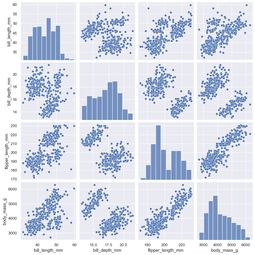
The pairplot() function offers a similar blend of joint and marginal distributions. Rather than focusing on a single relationship, however, pairplot() uses a “small-multiple” approach to visualize the univariate distribution of all variables in a dataset along with all of their pairwise relationships:

As with jointplot() / JointGrid , using the underlying PairGrid directly will afford more flexibility with only a bit more typing:

Визуализация одномерных данных в Python

Построение графика одной переменной кажется простой задачей. Но насколько это просто в действительности — эффективно отобразить данные со всего одним измерением? Долгое время я обходился стандартной гистограммой, которая показывает расположение значений, разброс и форму распределения данных (нормальное, скошенное, двухпиковое и др). Но недавно я столкнулся со случаем, когда гистограмма не помогла. И тогда понял, что настало время узнать больше о построении графиков. Я нашёл в сети отличную бесплатную книгу о визуализации данных и попробовал некоторые методы. Я решил, что (и мне, и другим людям) будет полезно, если я поделюсь этими знаниями и составлю руководство по построению на Python гистограмм и их крайне полезной альтернативы — графиков распределения плотности (density plots). Подробности — к старту нашего курса по анализу данных.

Я подробно рассмотрю применение гистограмм и графиков распределения в Python при помощи библиотек matplotlib и seaborn. На протяжении всего руководства исследуем набор реальных данных, потому что богатство доступных в сети материалов не даёт права отказываться от них! Покажем данные NYCflights13 с более чем 300000 наблюдений за авиарейсами из Нью-Йорка в 2013 году. Сосредоточимся на отображении одной переменной — задержки прибытия рейсов в минутах. Весь код этой статьи — в Jupyter Notebook на GitHub.

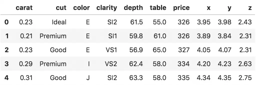
Перед построением графика всегда полезно изучить данные. Считаем данные во фрейм данных pandas и отобразим первые 10 строк:

Задержки рейсов указаны в минутах. Отрицательные значения означают, что самолёт совершил посадку с опережением графика (они часто его опережают в те самые дни, когда мы никуда не летим!) Всего у нас более 300000 рейсов. Наименьшая задержка составляет минус шестьдесят минут, наибольшая — сто двадцать минут. В другом столбце — названия авиалиний для сравнения.

Гистограммы

Разумно начать изучение данных с построения гистограммы. При построении гистограммы переменная делится на бины, точки данных подсчитываются в каждом бине, эти бины откладываются по оси x. По оси y откладывается число объектов. Здесь бины отражают диапазон времени задержки рейса, а по y откладывается число рейсов, попавшее в этот интервал. Важнейший параметр гистограммы — ширина бина (binwidth). Всегда стоит попробовать разную ширину и выбрать самую подходящую.

В Python базовую гистограмму может построить или matplotlib, или seaborn. В приведённом ниже коде показаны вызовы функций в обеих библиотеках, которые создают эквивалентные графики. При вызове функции plot мы указываем ширину бина, выраженную в числе бинов. Для этого графика я использую бины длиной 5 минут, что означает, что количество бинов будет равно диапазону данных (от -60 до 120 минут), делённому на ширину бина, 5 минут ( bins = int(180/5) ).

Для базовых гистограмм я использовал бы код matplotlib, поскольку он проще. Но в нашем примере для создания разных распределений мы воспользуемся функцией seaborn distplot . Она хорошо подходит для знакомства с разными вариантами.

Почему я взял за ширину бина 5 минут? Чтобы найти оптимальное значение, нужно попробовать разные варианты! Ниже я привожу код для создания такого же графика в matplotlib с различными значениями ширины бина. В конечном счёте нет верного или неверного ответа на вопрос о его ширине. Я выбрал 5 минут, потому что считаю, что это значение лучше всего отражает распределение.

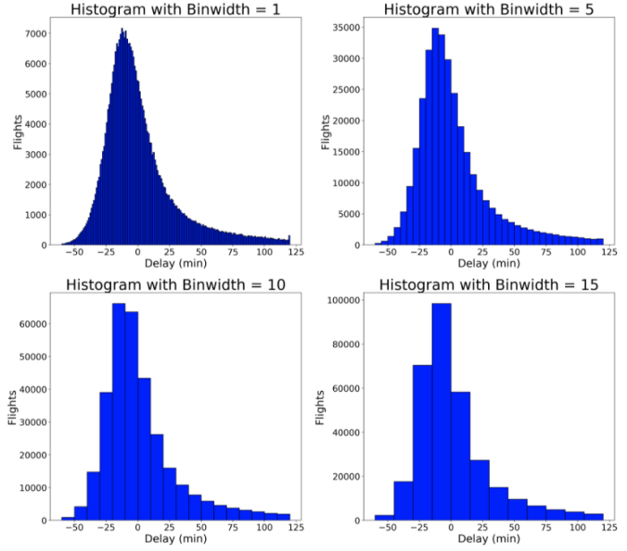
Ширина бина существенно влияет на вид графика. Слишком узкие бины загромождают его, а слишком широкие скрывают нюансы данных. Matplotlib выбирает оптимальную ширину бина автоматически, однако я предпочитаю выбирать значение вручную, перебирая варианты. Поскольку здесь нет ни единственно верного, ни заведомо неправильного выбора, попробуйте разные варианты и посмотрите, какой из них лучше всего подходит к вашему набору данных.

Когда гистограммы бесполезны

Гистограммы отлично подходят для начала исследования одной переменной, взятой из одной категории. Тем не менее, когда мы хотим сравнить распределения одной переменной по нескольким категориям, гистограммы не всегда удобны для восприятия. Например, если мы хотим сравнить распределения задержек прибытия рейсов разных авиалиний, построение гистограмм на одном графике плохо подходит для этой цели:

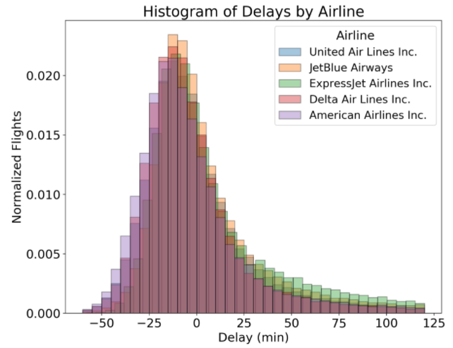
(Заметим, что ось y нормализована с учётом различий в количестве рейсов разных авиалиний. Для этого мы используем аргумент norm_hist = True при вызове функции sns.distplot ).

Пользы от такого графика мало! Перекрытие линий делает сравнение авиалиний практически невыполнимой задачей. Рассмотрим варианты решения этой задачи.

Вариант 1. Сравнительные гистограммы (Side-by-Side Histograms)

Вместо наложения гистограмм друг на друга мы можем расположить их рядом. Для этого создадим списки (list) задержек рейсов по авиалиниям, а затем передадим вызываемой функции plt.hist список таких списков. Разным авиалиниям мы присвоим разные цвета (color) и наименования (name), чтобы их проще было отличить друг от друга. Всё это, начиная с создания списков, делает вот такой код:

По умолчанию при передаче списка списков matplotlib размещает столбцы вплотную. В данном случае я изменил ширину бина до 15 минут, чтобы не перегружать график. Но даже с такой модификацией этот график неэффективен. Слишком много информации нужно обрабатывать одновременно, положение столбцов не совпадает с их метками, и сравнить распределения данных по авиалиниям всё равно сложно. Построение графика предполагает простоту интерпретации зрителем. Нам это не удалось! Давайте рассмотрим второй вариант решения.

Вариант 2. Столбчатые графики (Stacked Bars)

Вместо построения столбцов данных рядом мы можем расположить их друг над другом при помощи параметра stacked = True при вызове гистограммы:

Этот вариант ничуть не лучше! В каждом бине представлены доли всех авиалиний, однако сравнить их всё ещё невозможно. Вот например, у кого больше доля в бине от -15 до 0 минут: у United Air Lines или же у JetBlue Airlines? Я этого пока не знаю и аудитория тоже. И вообще, я не фанат столбчатых диаграмм. Они обычно трудны для понимания. (Полезными они могут быть лишь в отдельных случаях, например при визуализации соотношений). Ни один из этих гистограммных графиков не приблизил нас к решению. Настало время попробовать графики распределения.

Графики распределения (Density Plots)

Для начала — что это за графики? График распределения можно назвать непрерывным сглаженным аналогом гистограммы. Самый распространённый вариант построения такого графика — ядерная оценка плотности. В этом методе для каждой точки данных строится непрерывная кривая — ядро. Все эти кривые складываются вместе, чтобы получить единую гладкую оценку плотности. Чаще всего используется гауссово ядро (которое даёт колоколообразную кривую Гаусса в каждой точке данных). Если вы, как и я, находите это описание немного запутанным, взгляните на следующий график:

Ядерная оценка плотности (Источник)

Каждый чёрный вертикальный штрих у оси x представляет точку данных. Отдельные ядра (в данном случае — гауссовы) построены над каждой точкой красными пунктирными линиями. Их суммирование даёт общий график распределения, показанный сплошной синей линией.

По оси x здесь, как и на гистограмме, откладывается значение переменной. Но что показывает ось y? Ось y на графике плотности — это функция плотности вероятности для ядерной оценки плотности. Нужно помнить, что это именно плотность вероятности, а не сама вероятность. Разница между ними заключается в том, что плотность вероятности — это вероятность на единицу по оси x. Для преобразования этих данных в обычную вероятность нам нужно найти площадь под кривой для определённого интервала на оси x. Несколько смущает то, что поскольку это плотность вероятности, а не вероятность, ось y может принимать значения больше единицы. Единственное требование к графику плотности — чтобы общая площадь под кривой интегрировалась в единицу. Я привык рассматривать ось y на графике распределения как величину, применимую только для относительных сравнений между категориями.

Графики распределения в Seaborn

При построении графиков распределения в seaborn можно использовать функцию distplot или kdeplot . Я снова использую distplot , ведь он строит несколько распределений одним вызовом функции. Например, можно построить график распределения задержек всех рейсов поверх соответствующей гистограммы:

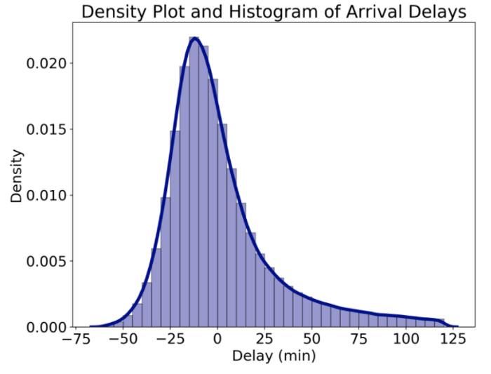
График распределения и гистограмма, построенные при помощи seaborn

Кривая — график распределения, который, по сути, является сглаженным аналогом гистограммы. По оси y откладывается плотность. Гистограмма по умолчанию нормализована. Поэтому её масштаб по оси y соответствует масштабу графика распределения.

У графика распределения есть величина, аналогичная ширине бина в гистограмме. Её называют шириной полосы пропускания (bandwidth). Эта величина позволяет изменить отдельные ядра и значительно влияет на общий вид графика. Библиотека построения графиков (plotting library) позволяет выбрать ширину полосы пропускания (по умолчанию используется «оценка по Скотту» (scott)). В отличие от гистограмм здесь я обычно полагаюсь на значение по умолчанию. Тем не менее ничто не мешает нам попробовать разную ширину полосы и выбрать оптимальную. Значение по умолчанию на этом графике, ‘scott’, действительно выглядит как наилучший вариант.

График распределения плотностей, показывающий различные полосы пропускания

Заметим, что с увеличением полосы пропускания распределение становится более сглаженным. Мы также видим, что, несмотря на ограничение данных от -60 до 120 минут, график плотности выходит за эти пределы. Это одна из возможных проблем графика плотности. Поскольку мы строим распределение в каждой точке данных, генерируемые данные могут выходить за рамки исходного диапазона. Таким образом, мы получаем на оси x нереалистичные значения, которых не было в исходном наборе данных! Мы также можем изменить ядро, что, в свою очередь, изменит распределение в каждой точке. Тем не менее в большинстве случаев ядро Гаусса по умолчанию и стандартная оценка полосы пропускания работают хорошо.

Вариант 3. График распределения

Теперь мы знаем, что представляет собой график распределения плотностей. Посмотрим, поможет ли он визуализировать задержки рейсов разных авиалиний. Чтобы показать эти распределения на одном графике, мы можем перебрать все авиалинии, каждый раз вызывая distplot . При этом мы присвоим параметру kde (kernel density estimate, ядерная оценка плотности) значение True, а параметру hist (гистограмма) — значение False. Код для построения графика распределения для множества авиалиний приведён ниже:

Наконец-то мы нашли эффективное решение! Этот график в меньшей степени загромождён, что позволяет проводить сравнения. Получив желанный график, мы можем сделать вывод. Рейсы всех этих авиалиний задерживаются почти одинаково: нет в жизни счастья! Но в нашем наборе данных есть и другие авиалинии, и мы можем построить немного другой график, который покажет ещё один дополнительный параметр графиков распределения плотности — затенение графика (shading).

Графики распределения с затенением (Shaded Density Plots)

Заполнение графика распределения плотностей позволяет нам различать перекрывающиеся распределения. Этот подход не всегда оправдан, но он может подчеркнуть разницу распределений. Чтобы затенять графики плотности, мы передаём shade = True в аргументе kde_kws при вызове функции distplot .

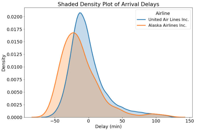
Затенять или не затенять — вот в чём вопрос… И ответ на него зависит от решаемой задачи! В нашем случае затенение не лишено смысла, поскольку помогает нам рассмотреть оба графика в области их перекрытия. Наконец, мы получили полезную информацию: рейсы Alaska Airlines показывают тенденцию к опережению графика чаще, чем United Airlines. Теперь вы знаете, чьи рейсы выбирать!

Штрих-диаграммы (Rug Plots)

Если вы хотите увидеть каждое значение в распределении, а не только сглаженный график плотности, вам также пригодится штрих-диаграмма.

Она показывает каждую точку на оси x и визуализирует все исходные значения. Преимущество использования distplot в seaborn — возможность добавления штрих-диаграммы при вызове rug = True с одним параметром (и небольшим форматированием).

Если точек данных много, штрих-диаграмма становится слишком сложной, однако она полезна в некоторых проектах, так как позволяет увидеть каждую точку данных. Штрих-диаграмма также наглядно показывает, как график распределения «создаёт» данные там, где их нет. Это связано с распределением ядерной оценки плотности в каждой точке данных. Это распределение может выходить за рамки начального диапазона данных, создавая впечатление, что некоторые рейсы Alaska Airlines прибывают и раньше и позже, чем в действительности. Нужно помнить об этой иллюзии и информировать о ней аудиторию!

Заключение

Смею надеяться, что в этом посте я перечислил набор полезных для вас вариантов визуализации значений одной переменной для одной и более категорий. Мы могли бы построить и другие одномерные («однопеременные») графики: эмпирические графики кумулятивной плотности (empirical cumulative density plots) и графики квантиль-квантиль (quantile-quantile plots). Однако в этой статье остановимся на гистограммах и графиках распределения (со штрих-диаграммами!). Если даже эти варианты кажутся вам слишком сложными, не отчаивайтесь. После некоторой практики вам станет проще сделать правильный выбор. Если потребуется, вы всегда можете обратиться за помощью. Более того, часто оптимального выбора не существует, а «верное» решение зависит и от личных предпочтений, и от цели визуализации данных. Но, какой бы график вы ни выбрали, вы всегда сможете построить его же Python! Визуальная подача доходчива, а зная все возможные варианты, мы всегда сможем выбрать наилучший график для нашего набора данных.

Любая обратная связь и конструктивная критика приветствуются. Меня можно найти в Twitter @koehrsen_will.

Научим вас аккуратно работать с данными, чтобы вы прокачали карьеру и стали востребованным IT-специалистом:

Statistical Distributions with Python Examples

A distribution provides a parameterised mathematical function that can be used to calculate the probability for any individual observation from the sample space.

The most common distributions are:

• Normal Distribution
• Student’s t-distribution
• Geometric distribution
• Bernoulli distribution
• Binomial distribution
• Poisson distribution
• Lognormal distribution

Density Functions

Distribution are usually described in terms of their density functions:

• PDF (Probability Density Function) is used to calculate the likelihood of a given observation in a distribution and can be represented as follow.

• CDF (Cumulative Density Function) calculates the cumulative likelihood for the observation and all prior observations in the sample space. Cumulative density function is a plot that goes from 0 to 1.

• PMF (Probability Mass Function) is a function that gives the probability that a discrete random variable is exactly equal to some value. It differs from a PDF because the latter is associated with continuous random variables and it needs to be integrated over an interval in order to yield a probability. We therefore refer to PMF when touching upon discrete distributions — in this case — Bernoulli, Binomial, and Geometric.

There are other probability functions in statistics and a more in-depth explanation can be found here: https://www.itl.nist.gov/div898/handbook/eda/section3/eda362.htm.

Gaussian Distribution aka Normal Distribution

A mong all the distributions we see in practice the Gaussian distribution is the most common. Variables such as SAT scores and heights of female/male adult follow this distribution. The normal distribution always describes a symmetric, unimodal, bell-shaped curve. The distribution depends on two parameters, �� and ��, therefore we can write it as ��(��,��). When ��=0 and ��=1, then in that case we talk about Standard Normal distribution.

The probability density function of the Normal Distribution is somewhat a complex formula:

Luckily for us we can refer to it through some tables with values depending on parameters �� and ��, or using R or Python. Below a Python snippet you can use in order to create a Normal Distribution with ��=0 and ��=1.

Gaussian Distribution’s PDF in python

Gaussian Distribution’s CDF in python

Practical Example

How many people have an SAT score below Simone’s score of 1300 if population have μ=1100 and σ = 200?

You can solve this using scipy.stats in python:

You can also solve the above question in a different manner using the standardised Z-score. How to achieve that? Using the formula to find Z:

Z = (x-��)/�� = (1300–1100) / 200 = 1
Now you need to find out the probability distribution associated with Z=1. You can use either some pre-calculated tables or Python (or R). With Python you can use the following snippet:

Student’s t-Distribution

S tudent distribution is used to estimating the mean of a normally-distributed population in situations where the sample size is small and the population’s standard deviation is unknown. The t-distribution is symmetric and bell-shaped, like the Normal distribution, however it has heavier tails, meaning it is more prone to producing values that fall far from its mean. t-distribution is characterised by the degrees of freedom which equals to ��=��−1 (�� is pronounced as nu).

Student t Distribution-PDF

As you can see from the graph above, the bigger the degree of freedom, the slimmer are the tails. This also means that with �� increasing the t-distribution approximates more and more to the Normal distribution. More on the subject at the following link: https://mathworld.wolfram.com/Studentst-Distribution.html.

Geometric Distribution

H ow many visits should we expect from a user before making a purchase? How long should we expect to flip a coin until it turns up heads? These can be expressed through a Geometric Distribution.

Each trial has two possible outcomes, purchase or not purchase for the first example, and heads or tails in the second. This is represented through a Bernoulli Distribution in statistics. Let’s first see what Bernoulli defines.

Bernoulli Distribution

If X is a random variable that takes value 1 with probability of success p and 0 with probability 1-p, then X is a Bernoulli random variable with mean and standard deviation as follow:

Suppose, on a specific e-commerce page a user make a purchase with probability 10%, based on historical data. Each user can be thought as a trial. The probability of success in this case is p = 0.1, whereas the probability of a failure is denoted as q = 1 — p = 0.9.

Geometric Distribution in Detail

If the probability of a success in one trial is p and the probability of a failure is 1 — p, then the probability of finding the first success in the n(th) trial is as follow:

And expected value, variance, and standard deviation are:

You may be interested on creating a series of random variates based on the parameters of your distribution. In our previous example, we assumed that the probability of converting for a user was p = 0.1. You can use Python to create those variates:

If you are interested on plotting the probability mass function (because it is a discrete random variable) for the distribution with parameter p = 0.1, then you can to use the following snippet:

The cumulative density function for the same example above is represented by:

As represented above, the cumulative density function increase step by step. Indeed it is simply the sum of all the previous probability until that point (the sum of each probability of the PMF till that point to be precise). This also means that the cumulative probability of a user making a purchase gets bigger users after users. E.g. if we know that our users make a purchase with p = 0.1, we know that we expect to drive a purchase within around 10 users — on average — if you are far off from it…well, you better have a look at your last release :).

Practical Example

What is the probability that the 5th user landing on the e-commerce page today will make a purchase? Probability of a user converting, based on historical data, p=0.1.

What is the probability that a user will make a purchase within the next 7 trials/users visiting the e-commerce page?

Binomial Distribution

T he Binomial Distribution is used to describe the number of success in a fixed number of trials. This is different from the geometric distribution, which describes the number of trials we must wait before we observe a success. We need to check that four conditions are respected first:

1. Trials are independent.
2. The number of trials, n, is fixed.
3. Each trial outcome can be classified as a success or failure.
4. The probability of a success, p, is the same for each trial.

Suppose the probability of a singe trial being a success is p. Then the probability of observing exactly k success in n independent trials is given by:

Mean, variance and standard deviation are:

Probability Mass Function — Binomial Distribution

With it we can understand what is the probability of having 1, 2, 3 purchases from our users landing in the e-commerce page.

Practical Example

Based on the previous example, regarding the probability of a user purchasing in an e-commerce page.

What is the probability of 2 users making a purchase out of 20 users landing on the page? p=0.1, k= 2, n=20.

You could infer it from the graph above, it is around 25%, but if you want to have a precise value you can calculate it directly with python:

What is the probability of hiring 2 persons out of 50 candidates if you know that on average your company hire 1 out of 50 candidates?

Note: The binomial distribution with probability of success p is nearly normal when the sample size n is sufficiently large that np and n(1-p) are both at least 10. This means we calculate our expected value and standard deviation:

And after we find Z, and we can check its probability (as showed at the beginning of the article):

Poisson Distribution

T he Poisson distribution is often useful for estimating the number of events in a large population over a unit of time. In general for applying Poisson the events need to be independent, the average rate (event per time period) is constant, and two events cannot occur at the same time. The average rate is �� (lambda). Using the rate, we can describe the probability of observing exactly k events in a unit of time.

Following a Poisson distribution are variables like visitors on a website, customer calling an help center, movements in stock price. For example, if you want to know the how many users will land on a page in the next 60 seconds, that can be modelled by a Poisson distribution and the PMF describing it is as follow:

Practical Examples

If you want to know what is the probability of observing 55 users in the next 60 second, when �� = 45/m (45 users per minute), then:

If you want to know the probability of observing more than 55 users in the next 60 seconds, when �� = 45/m (45 users per minute):

What is the probability of hiring 2 persons out of 60 candidates if you have p=0.02?

Poisson Distribution — PMF

Lognormal Distribution

A lognormal distribution is a probability distribution with a normally distributed logarithm. Right skewed distributions with low mean values, large variance, and all positive values often fit this distribution. Example of lognormal distribution in nature are the amount of rainfall, milk production by cows, and for most natural growth processes, where the growth rate is independent of size.

Matplotlib Histogram – How to Visualize Distributions in Python

Matplotlib histogram is used to visualize the frequency distribution of numeric array by splitting it to small equal-sized bins. In this article, we explore practical techniques that are extremely useful in your initial data analysis and plotting.

Content

1. What is a histogram?
2. How to plot a basic histogram in python?
3. Histogram grouped by categories in same plot
4. Histogram grouped by categories in separate subplots
5. Seaborn Histogram and Density Curve on the same plot
6. Histogram and Density Curve in Facets
7. Difference between a Histogram and a Bar Chart
8. Practice Exercise
9. Conclusion

1. What is a Histogram?

A histogram is a plot of the frequency distribution of numeric array by splitting it to small equal-sized bins.

If you want to mathemetically split a given array to bins and frequencies, use the numpy histogram() method and pretty print it like below.

The output of above code looks like this:

The above representation, however, won’t be practical on large arrays, in which case, you can use matplotlib histogram.

2. How to plot a basic histogram in python?

The pyplot.hist() in matplotlib lets you draw the histogram. It required the array as the required input and you can specify the number of bins needed. Histogram

3. Histogram grouped by categories in same plot

You can plot multiple histograms in the same plot. This can be useful if you want to compare the distribution of a continuous variable grouped by different categories.

Let’s use the diamonds dataset from R’s ggplot2 package. Diamonds Table

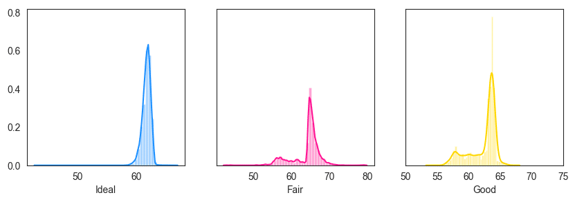
Let’s compare the distribution of diamond depth for 3 different values of diamond cut in the same plot.

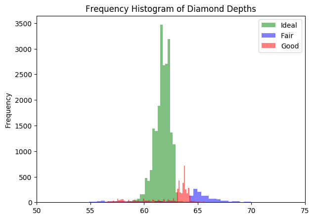
Multi Histogram

Well, the distributions for the 3 differenct cuts are distinctively different. But since, the number of datapoints are more for Ideal cut, the it is more dominant.

So, how to rectify the dominant class and still maintain the separateness of the distributions?

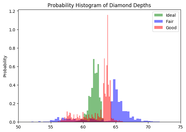
You can normalize it by setting density=True and stacked=True . By doing this the total area under each distribution becomes 1. Multi Histogram 2

4. Histogram grouped by categories in separate subplots

The histograms can be created as facets using the plt.subplots()

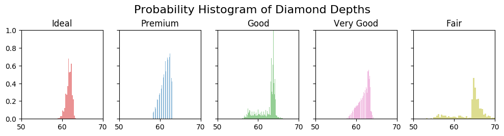
Below I draw one histogram of diamond depth for each category of diamond cut . It’s convenient to do it in a for-loop. Histograms Facets

5. Seaborn Histogram and Density Curve on the same plot

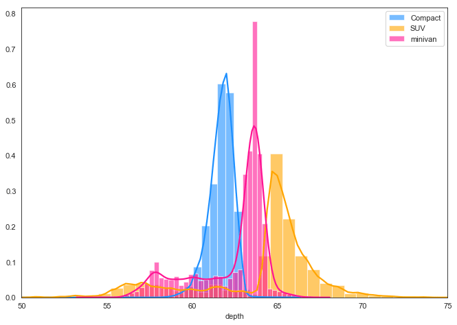
If you wish to have both the histogram and densities in the same plot, the seaborn package (imported as sns ) allows you to do that via the distplot() . Since seaborn is built on top of matplotlib, you can use the sns and plt one after the other. Histograms Density

6. Histogram and Density Curve in Facets

The below example shows how to draw the histogram and densities ( distplot ) in facets. Histogram Density Facets

7. Difference between a Histogram and a Bar Chart

A histogram is drawn on large arrays. It computes the frequency distribution on an array and makes a histogram out of it.

On the other hand, a bar chart is used when you have both X and Y given and there are limited number of data points that can be shown as bars. 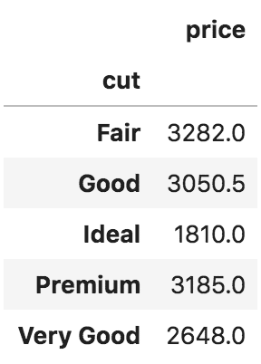Diamonds_Cut 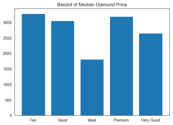Barplots

8. Practice Exercise

Create the following density on the sepal_length of iris dataset on your Jupyter Notebook. Show Solution

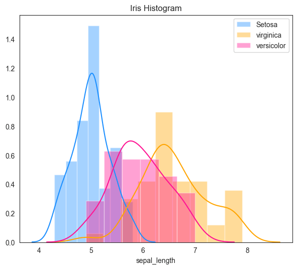
Iris Histograms