Pyplot tutorial#
An introduction to the pyplot interface. Please also see Quick start guide for an overview of how Matplotlib works and Matplotlib Application Interfaces (APIs) for an explanation of the trade-offs between the supported user APIs.
Introduction to pyplot#
matplotlib.pyplot is a collection of functions that make matplotlib work like MATLAB. Each pyplot function makes some change to a figure: e.g., creates a figure, creates a plotting area in a figure, plots some lines in a plotting area, decorates the plot with labels, etc.
In matplotlib.pyplot various states are preserved across function calls, so that it keeps track of things like the current figure and plotting area, and the plotting functions are directed to the current axes (please note that "axes" here and in most places in the documentation refers to the axes part of a figure and not the strict mathematical term for more than one axis).
The implicit pyplot API is generally less verbose but also not as flexible as the explicit API. Most of the function calls you see here can also be called as methods from an Axes object. We recommend browsing the tutorials and examples to see how this works. See Matplotlib Application Interfaces (APIs) for an explanation of the trade-off of the supported user APIs.
Generating visualizations with pyplot is very quick:

You may be wondering why the x-axis ranges from 0-3 and the y-axis from 1-4. If you provide a single list or array to plot , matplotlib assumes it is a sequence of y values, and automatically generates the x values for you. Since python ranges start with 0, the default x vector has the same length as y but starts with 0; therefore, the x data are [0, 1, 2, 3] .
plot is a versatile function, and will take an arbitrary number of arguments. For example, to plot x versus y, you can write:

Formatting the style of your plot#
For every x, y pair of arguments, there is an optional third argument which is the format string that indicates the color and line type of the plot. The letters and symbols of the format string are from MATLAB, and you concatenate a color string with a line style string. The default format string is ‘b-‘, which is a solid blue line. For example, to plot the above with red circles, you would issue

See the plot documentation for a complete list of line styles and format strings. The axis function in the example above takes a list of [xmin, xmax, ymin, ymax] and specifies the viewport of the axes.
If matplotlib were limited to working with lists, it would be fairly useless for numeric processing. Generally, you will use numpy arrays. In fact, all sequences are converted to numpy arrays internally. The example below illustrates plotting several lines with different format styles in one function call using arrays.

Plotting with keyword strings#
There are some instances where you have data in a format that lets you access particular variables with strings. For example, with numpy.recarray or pandas.DataFrame .
Matplotlib allows you to provide such an object with the data keyword argument. If provided, then you may generate plots with the strings corresponding to these variables.

Plotting with categorical variables#
It is also possible to create a plot using categorical variables. Matplotlib allows you to pass categorical variables directly to many plotting functions. For example:

Controlling line properties#
Lines have many attributes that you can set: linewidth, dash style, antialiased, etc; see matplotlib.lines.Line2D . There are several ways to set line properties
Use keyword arguments:
Use the setter methods of a Line2D instance. plot returns a list of Line2D objects; e.g., line1, line2 = plot(x1, y1, x2, y2) . In the code below we will suppose that we have only one line so that the list returned is of length 1. We use tuple unpacking with line, to get the first element of that list:
Use setp . The example below uses a MATLAB-style function to set multiple properties on a list of lines. setp works transparently with a list of objects or a single object. You can either use python keyword arguments or MATLAB-style string/value pairs:
Here are the available Line2D properties.
antialiased or aa
a matplotlib.transform.Bbox instance
a Path instance and a Transform instance, a Patch
any matplotlib color
the hit testing function
[ ‘butt’ | ’round’ | ‘projecting’ ]
[ ‘miter’ | ’round’ | ‘bevel’ ]
sequence of on/off ink in points
(np.array xdata, np.array ydata)
a matplotlib.figure.Figure instance
linestyle or ls
linewidth or lw
float value in points
markeredgecolor or mec
any matplotlib color
markeredgewidth or mew
float value in points
markerfacecolor or mfc
any matplotlib color
markersize or ms
[ None | integer | (startind, stride) ]
used in interactive line selection
the line pick selection radius
[ ‘butt’ | ’round’ | ‘projecting’ ]
[ ‘miter’ | ’round’ | ‘bevel’ ]
a matplotlib.transforms.Transform instance
To get a list of settable line properties, call the setp function with a line or lines as argument
Working with multiple figures and axes#
MATLAB, and pyplot , have the concept of the current figure and the current axes. All plotting functions apply to the current axes. The function gca returns the current axes (a matplotlib.axes.Axes instance), and gcf returns the current figure (a matplotlib.figure.Figure instance). Normally, you don’t have to worry about this, because it is all taken care of behind the scenes. Below is a script to create two subplots.

The figure call here is optional because a figure will be created if none exists, just as an Axes will be created (equivalent to an explicit subplot() call) if none exists. The subplot call specifies numrows, numcols, plot_number where plot_number ranges from 1 to numrows*numcols . The commas in the subplot call are optional if numrows*numcols<10 . So subplot(211) is identical to subplot(2, 1, 1) .
You can create an arbitrary number of subplots and axes. If you want to place an Axes manually, i.e., not on a rectangular grid, use axes , which allows you to specify the location as axes([left, bottom, width, height]) where all values are in fractional (0 to 1) coordinates. See Axes Demo for an example of placing axes manually and Multiple subplots for an example with lots of subplots.
You can create multiple figures by using multiple figure calls with an increasing figure number. Of course, each figure can contain as many axes and subplots as your heart desires:
You can clear the current figure with clf and the current axes with cla . If you find it annoying that states (specifically the current image, figure and axes) are being maintained for you behind the scenes, don’t despair: this is just a thin stateful wrapper around an object-oriented API, which you can use instead (see Artist tutorial )
If you are making lots of figures, you need to be aware of one more thing: the memory required for a figure is not completely released until the figure is explicitly closed with close . Deleting all references to the figure, and/or using the window manager to kill the window in which the figure appears on the screen, is not enough, because pyplot maintains internal references until close is called.
Working with text#
text can be used to add text in an arbitrary location, and xlabel , ylabel and title are used to add text in the indicated locations (see Text in Matplotlib Plots for a more detailed example)

All of the text functions return a matplotlib.text.Text instance. Just as with lines above, you can customize the properties by passing keyword arguments into the text functions or using setp :
These properties are covered in more detail in Text properties and layout .
Using mathematical expressions in text#
Matplotlib accepts TeX equation expressions in any text expression. For example to write the expression \(\sigma_i=15\) in the title, you can write a TeX expression surrounded by dollar signs:
The r preceding the title string is important — it signifies that the string is a raw string and not to treat backslashes as python escapes. matplotlib has a built-in TeX expression parser and layout engine, and ships its own math fonts — for details see Writing mathematical expressions . Thus, you can use mathematical text across platforms without requiring a TeX installation. For those who have LaTeX and dvipng installed, you can also use LaTeX to format your text and incorporate the output directly into your display figures or saved postscript — see Text rendering with LaTeX .
Annotating text#
The uses of the basic text function above place text at an arbitrary position on the Axes. A common use for text is to annotate some feature of the plot, and the annotate method provides helper functionality to make annotations easy. In an annotation, there are two points to consider: the location being annotated represented by the argument xy and the location of the text xytext . Both of these arguments are (x, y) tuples.

In this basic example, both the xy (arrow tip) and xytext locations (text location) are in data coordinates. There are a variety of other coordinate systems one can choose — see Basic annotation and Advanced annotation for details. More examples can be found in Annotating Plots .
Logarithmic and other nonlinear axes#
matplotlib.pyplot supports not only linear axis scales, but also logarithmic and logit scales. This is commonly used if data spans many orders of magnitude. Changing the scale of an axis is easy:
An example of four plots with the same data and different scales for the y-axis is shown below.

It is also possible to add your own scale, see matplotlib.scale for details.
Total running time of the script: ( 0 minutes 4.003 seconds)
Python Matplotlib Guide — Learn Matplotlib Library with Examples

In my previous blog, I discussed a numerical library of python called Python NumPy. In this blog, I will be talking about another library, Python Matplotlib. matplotlib.pyplot is a python package used for 2D graphics. Below is the sequence in which I will be covering all the topics of python matplotlib:
- What Is Python Matplotlib?
- Types Of Plots
– Bar Graph
– Histogram
– Scatter Plot
– Area Plot
– Pie Chart - Working With Multiple Plots
What Is Python Matplotlib?
matplotlib.pyplot is a plotting library used for 2D graphics in python programming language. It can be used in python scripts, shell, web application servers and other graphical user interface toolkits.
There are several toolkits that are available that extend python matplotlib functionality. Some of them are separate downloads, others can be shipped with the matplotlib source code but have external dependencies.
- Basemap: It is a map plotting toolkit with various map projections, coastlines, and political boundaries.
- Cartopy: It is a mapping library featuring object-oriented map projection definitions, and arbitrary point, line, polygon and image transformation capabilities.
- Excel tools: Matplotlib provides utilities for exchanging data with Microsoft Excel.
- Mplot3d: It is used for 3-D plots.
- Natgrid: It is an interface to the natgrid library for irregular gridding of the spaced data.
Next, let us move forward in this blog and explore different types of plots available in python matplotlib.
Types of Plots
There are various plots which can be created using python matplotlib. Some of them are listed below:
I will demonstrate each one of them in detail.
But before that, let me show you very basic codes in python matplotlib in order to generate a simple graph.
Output –
So, with three lines of code, you can generate a basic graph using python matplotlib. Simple, isn’t it?
Let us see how can we add title and labels to our graph created by python matplotlib library to bring in more meaning to it. Consider the below example:
Output –
You can even try many styling techniques to create a better graph. What if you want to change the width or color of a particular line or what if you want to have some grid lines, there you need styling! So, let me show you how to add style to a graph using python matplotlib. First, you need to import the style package from python matplotlib library and then use styling functions as shown in below code:
Output –
Next, in this python matplotlib blog, we will understand different kinds of plots. Let’s start with the bar graph!
Bar Graph
First, let us understand why do we need a bar graph. A bar graph uses bars to compare data among different categories. It is well suited when you want to measure the changes over a period of time. It can be represented horizontally or vertically. Also, the important thing to keep in mind is that longer the bar, greater is the value. Now, let us practically implement it using python matplotlib.
Output –
In the above plot, I have displayed the comparison between the distance covered by two cars BMW and Audi over a period of 5 days. Next, let us move on to another kind of plot using python matplotlib — Histogram.
Histogram
Let me first tell you the difference between a bar graph and a histogram. Histograms are used to show a distribution whereas a bar chart is used to compare different entities. Histograms are useful when you have arrays or a very long list. Let’s consider an example where I have to plot the age of population with respect to the bin. Now, bin refers to the range of values that are divided into a series of intervals. Bins are usually created of the same size. In the below code, I have created the bins in the interval of 10 which means the first bin contains elements from 0 to 9, then 10 to 19 and so on.
Output –
As you can see in the above plot, we got age groups with respect to the bins. Our biggest age group is between 40 and 50.
Scatter Plot
Usually, we need scatter plots in order to compare variables, for example, how much one variable is affected by another variable to build a relation out of it. The data is displayed as a collection of points, each having the value of one variable which determines the position on the horizontal axis and the value of other variable determines the position on the vertical axis.
Consider the below example:
Output –
As you can see in the above graph, I have plotted two scatter plots based on the inputs specified in the above code. The data is displayed as a collection of points having ‘high-income low salary’ and ‘low-income high salary’.
Next, let us understand area plot or you can also say Stack plot using python matplotlib.
Area Plot
Area plots are pretty much similar to the line plot. They are also known as stack plots. These plots can be used to track changes over time for two or more related groups that make up one whole category. For example, let’s compile the work done during a day into categories, say sleeping, eating, working and playing. Consider the below code:
Output –
As we can see in the above image, we have time spent based on the categories. Therefore, area plot or stack plot is used to show trends over time, among different attributes. Next, let us move to our last yet most frequently used plot — Pie chart.
Pie Chart
A pie chart refers to a circular graph which is broken down into segments i.e. slices of pie. It is basically used to show the percentage or proportional data where each slice of pie represents a category. Let’s have a look at the below example:
Output –
In the above pie chart, I have divided the circle into 4 sectors or slices which represents the respective category (playing, sleeping, eating and working) along with the percentage they hold. Now, if you have noticed these slices adds up to 24 hrs, but the calculation of pie slices is done automatically for you. In this way, pie charts are really useful as you don’t have to be the one who calculates the percentage or the slice of the pie.
Next, in python matplotlib, let’s understand how to work with multiple plots.
Working With Multiple Plots
I have discussed about multiple types of plots in python matplotlib such as bar plot, scatter plot, pie plot, area plot etc. Now, let me show you how to handle multiple plots. For this, I have to import numpy module which I discussed in my previous blog on Python Numpy. Let me implement it practically, consider the below example.
Output-
The code is pretty much similar to the previous examples that you have seen but there is one new concept here i.e. subplot. The subplot() command specifies numrow, numcol, fignum which ranges from 1 to numrows*numcols. The commas in this command are optional if numrows*numcols<10. So subplot (221) is identical to subplot (2,2,1). Therefore, subplots help us to plot multiple graphs in which you can define it by aligning vertically or horizontally. In the above example, I have aligned it horizontally.
Apart from these, python matplotlib has some disadvantages. Some of them are listed below:
- They are heavily reliant on other packages, such as NumPy.
- It only works for python, so it is hard or impossible to be used in languages other than python. (But it can be used from Julia via PyPlot package).
We have come to an end of this python matplotlib tutorial. I have covered all the basics of matplotlib, so you can start practicing now. I hope you guys are clear about each and every aspect that I have discussed above.
If you wish to check out more articles on the market’s most trending technologies like Artificial Intelligence, DevOps, Ethical Hacking, then you can refer to Edureka’s official site.
Do look out for other articles in this series which will explain the various other aspects of Python and Data Science.
Quick start guide#
This tutorial covers some basic usage patterns and best practices to help you get started with Matplotlib.
A simple example#
Matplotlib graphs your data on Figure s (e.g., windows, Jupyter widgets, etc.), each of which can contain one or more Axes , an area where points can be specified in terms of x-y coordinates (or theta-r in a polar plot, x-y-z in a 3D plot, etc.). The simplest way of creating a Figure with an Axes is using pyplot.subplots . We can then use Axes.plot to draw some data on the Axes:

Note that to get this Figure to display, you may have to call plt.show() , depending on your backend. For more details of Figures and backends, see Creating, viewing, and saving Matplotlib Figures .
Parts of a Figure#
Here are the components of a Matplotlib Figure.
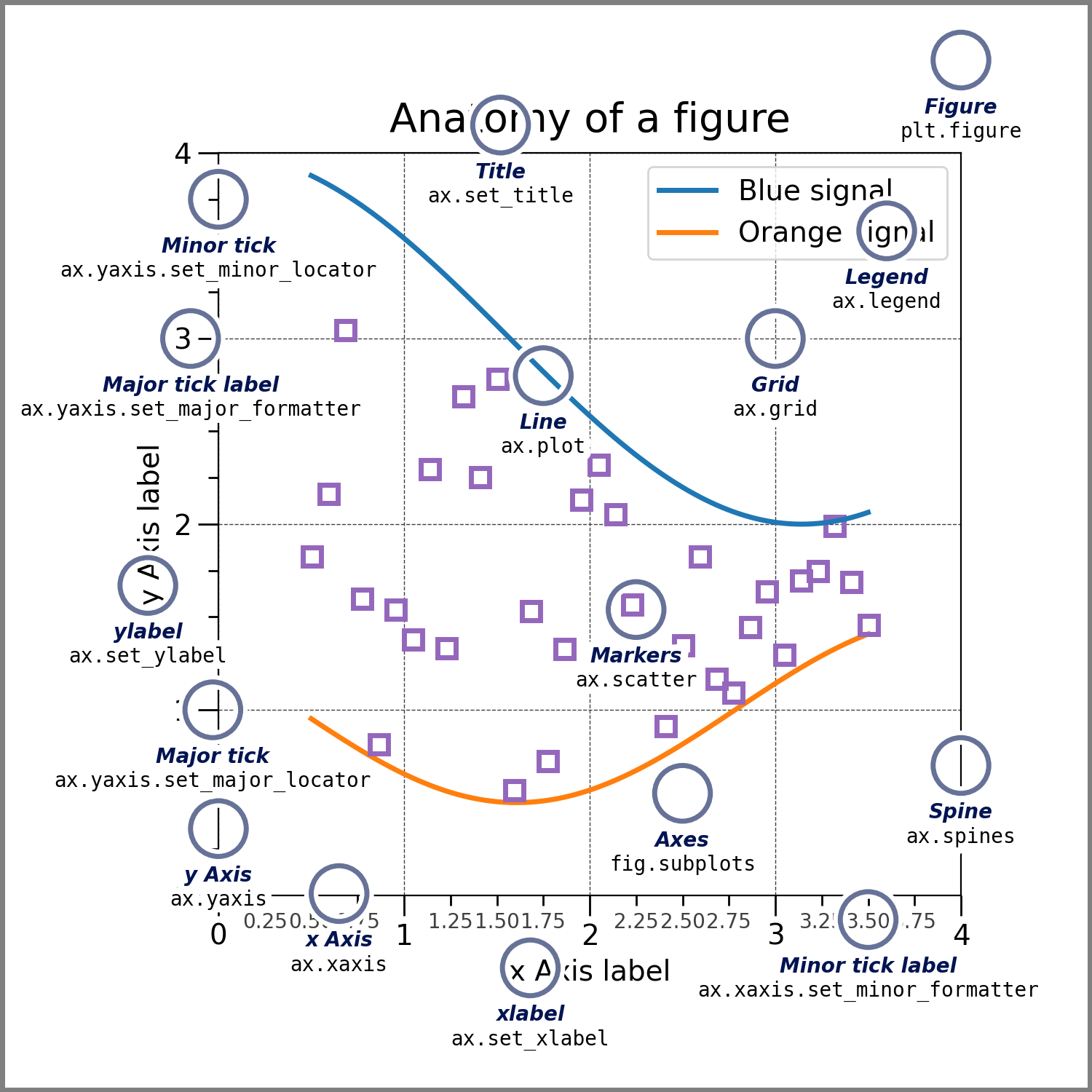
Figure #
The whole figure. The Figure keeps track of all the child Axes , a group of ‘special’ Artists (titles, figure legends, colorbars, etc), and even nested subfigures.
The easiest way to create a new Figure is with pyplot:
It is often convenient to create the Axes together with the Figure, but you can also manually add Axes later on. Note that many Matplotlib backends support zooming and panning on figure windows.
An Axes is an Artist attached to a Figure that contains a region for plotting data, and usually includes two (or three in the case of 3D) Axis objects (be aware of the difference between Axes and Axis) that provide ticks and tick labels to provide scales for the data in the Axes. Each Axes also has a title (set via set_title() ), an x-label (set via set_xlabel() ), and a y-label set via set_ylabel() ).
The Axes class and its member functions are the primary entry point to working with the OOP interface, and have most of the plotting methods defined on them (e.g. ax.plot() , shown above, uses the plot method)
These objects set the scale and limits and generate ticks (the marks on the Axis) and ticklabels (strings labeling the ticks). The location of the ticks is determined by a Locator object and the ticklabel strings are formatted by a Formatter . The combination of the correct Locator and Formatter gives very fine control over the tick locations and labels.
Artist #
Basically, everything visible on the Figure is an Artist (even Figure , Axes , and Axis objects). This includes Text objects, Line2D objects, collections objects, Patch objects, etc. When the Figure is rendered, all of the Artists are drawn to the canvas. Most Artists are tied to an Axes; such an Artist cannot be shared by multiple Axes, or moved from one to another.
Types of inputs to plotting functions#
Plotting functions expect numpy.array or numpy.ma.masked_array as input, or objects that can be passed to numpy.asarray . Classes that are similar to arrays (‘array-like’) such as pandas data objects and numpy.matrix may not work as intended. Common convention is to convert these to numpy.array objects prior to plotting. For example, to convert a numpy.matrix
Most methods will also parse an addressable object like a dict, a numpy.recarray , or a pandas.DataFrame . Matplotlib allows you to provide the data keyword argument and generate plots passing the strings corresponding to the x and y variables.

Coding styles#
The explicit and the implicit interfaces#
As noted above, there are essentially two ways to use Matplotlib:
Explicitly create Figures and Axes, and call methods on them (the "object-oriented (OO) style").
Rely on pyplot to implicitly create and manage the Figures and Axes, and use pyplot functions for plotting.
See Matplotlib Application Interfaces (APIs) for an explanation of the tradeoffs between the implicit and explicit interfaces.
So one can use the OO-style

or the pyplot-style:

(In addition, there is a third approach, for the case when embedding Matplotlib in a GUI application, which completely drops pyplot, even for figure creation. See the corresponding section in the gallery for more info: Embedding Matplotlib in graphical user interfaces .)
Matplotlib’s documentation and examples use both the OO and the pyplot styles. In general, we suggest using the OO style, particularly for complicated plots, and functions and scripts that are intended to be reused as part of a larger project. However, the pyplot style can be very convenient for quick interactive work.
You may find older examples that use the pylab interface, via from pylab import * . This approach is strongly deprecated.
Making a helper functions#
If you need to make the same plots over and over again with different data sets, or want to easily wrap Matplotlib methods, use the recommended signature function below.
which you would then use twice to populate two subplots:

Note that if you want to install these as a python package, or any other customizations you could use one of the many templates on the web; Matplotlib has one at mpl-cookiecutter
Styling Artists#
Most plotting methods have styling options for the Artists, accessible either when a plotting method is called, or from a "setter" on the Artist. In the plot below we manually set the color, linewidth, and linestyle of the Artists created by plot , and we set the linestyle of the second line after the fact with set_linestyle .

Colors#
Matplotlib has a very flexible array of colors that are accepted for most Artists; see the colors tutorial for a list of specifications. Some Artists will take multiple colors. i.e. for a scatter plot, the edge of the markers can be different colors from the interior:

Linewidths, linestyles, and markersizes#
Line widths are typically in typographic points (1 pt = 1/72 inch) and available for Artists that have stroked lines. Similarly, stroked lines can have a linestyle. See the linestyles example .
Marker size depends on the method being used. plot specifies markersize in points, and is generally the "diameter" or width of the marker. scatter specifies markersize as approximately proportional to the visual area of the marker. There is an array of markerstyles available as string codes (see markers ), or users can define their own MarkerStyle (see Marker reference ):

Labelling plots#
Axes labels and text#
set_xlabel , set_ylabel , and set_title are used to add text in the indicated locations (see Text in Matplotlib Plots for more discussion). Text can also be directly added to plots using text :

All of the text functions return a matplotlib.text.Text instance. Just as with lines above, you can customize the properties by passing keyword arguments into the text functions:
These properties are covered in more detail in Text properties and layout .
Using mathematical expressions in text#
Matplotlib accepts TeX equation expressions in any text expression. For example to write the expression \(\sigma_i=15\) in the title, you can write a TeX expression surrounded by dollar signs:
where the r preceding the title string signifies that the string is a raw string and not to treat backslashes as python escapes. Matplotlib has a built-in TeX expression parser and layout engine, and ships its own math fonts – for details see Writing mathematical expressions . You can also use LaTeX directly to format your text and incorporate the output directly into your display figures or saved postscript – see Text rendering with LaTeX .
Annotations#
We can also annotate points on a plot, often by connecting an arrow pointing to xy, to a piece of text at xytext:

In this basic example, both xy and xytext are in data coordinates. There are a variety of other coordinate systems one can choose — see Basic annotation and Advanced annotation for details. More examples also can be found in Annotating Plots .
Legends#
Often we want to identify lines or markers with a Axes.legend :

Legends in Matplotlib are quite flexible in layout, placement, and what Artists they can represent. They are discussed in detail in Legend guide .
Axis scales and ticks#
Each Axes has two (or three) Axis objects representing the x- and y-axis. These control the scale of the Axis, the tick locators and the tick formatters. Additional Axes can be attached to display further Axis objects.
Scales#
In addition to the linear scale, Matplotlib supplies non-linear scales, such as a log-scale. Since log-scales are used so much there are also direct methods like loglog , semilogx , and semilogy . There are a number of scales (see Scales for other examples). Here we set the scale manually:

The scale sets the mapping from data values to spacing along the Axis. This happens in both directions, and gets combined into a transform, which is the way that Matplotlib maps from data coordinates to Axes, Figure, or screen coordinates. See Transformations Tutorial .
Tick locators and formatters#
Each Axis has a tick locator and formatter that choose where along the Axis objects to put tick marks. A simple interface to this is set_xticks :

Different scales can have different locators and formatters; for instance the log-scale above uses LogLocator and LogFormatter . See Tick locators and Tick formatters for other formatters and locators and information for writing your own.
Plotting dates and strings#
Matplotlib can handle plotting arrays of dates and arrays of strings, as well as floating point numbers. These get special locators and formatters as appropriate. For dates:

For more information see the date examples (e.g. Date tick labels )
For strings, we get categorical plotting (see: Plotting categorical variables ).

One caveat about categorical plotting is that some methods of parsing text files return a list of strings, even if the strings all represent numbers or dates. If you pass 1000 strings, Matplotlib will think you meant 1000 categories and will add 1000 ticks to your plot!
Additional Axis objects#
Plotting data of different magnitude in one chart may require an additional y-axis. Such an Axis can be created by using twinx to add a new Axes with an invisible x-axis and a y-axis positioned at the right (analogously for twiny ). See Plots with different scales for another example.
Similarly, you can add a secondary_xaxis or secondary_yaxis having a different scale than the main Axis to represent the data in different scales or units. See Secondary Axis for further examples.

Color mapped data#
Often we want to have a third dimension in a plot represented by a colors in a colormap. Matplotlib has a number of plot types that do this:

Colormaps#
These are all examples of Artists that derive from ScalarMappable objects. They all can set a linear mapping between vmin and vmax into the colormap specified by cmap. Matplotlib has many colormaps to choose from ( Choosing Colormaps in Matplotlib ) you can make your own ( Creating Colormaps in Matplotlib ) or download as third-party packages.
Normalizations#
Sometimes we want a non-linear mapping of the data to the colormap, as in the LogNorm example above. We do this by supplying the ScalarMappable with the norm argument instead of vmin and vmax. More normalizations are shown at Colormap Normalization .
Colorbars#
Adding a colorbar gives a key to relate the color back to the underlying data. Colorbars are figure-level Artists, and are attached to a ScalarMappable (where they get their information about the norm and colormap) and usually steal space from a parent Axes. Placement of colorbars can be complex: see Placing Colorbars for details. You can also change the appearance of colorbars with the extend keyword to add arrows to the ends, and shrink and aspect to control the size. Finally, the colorbar will have default locators and formatters appropriate to the norm. These can be changed as for other Axis objects.
Working with multiple Figures and Axes#
You can open multiple Figures with multiple calls to fig = plt.figure() or fig2, ax = plt.subplots() . By keeping the object references you can add Artists to either Figure.
Multiple Axes can be added a number of ways, but the most basic is plt.subplots() as used above. One can achieve more complex layouts, with Axes objects spanning columns or rows, using subplot_mosaic .

More reading#
For more plot types see Plot types and the API reference , in particular the Axes API .
Total running time of the script: ( 0 minutes 8.602 seconds)
Визуализация данных с matplotlib
Библиотека matplotlib содержит большой набор инструментов для двумерной графики. Она проста в использовании и позволяет получать графики высокого качества. В этом разделе мы рассмотрим наиболее распространенные типы диаграмм и различные настройки их отображения.
Модуль matplotlib.pyplot предоставляет процедурный интерфейс к (объектно-ориентированной) библиотеке matplotlib, который во многом копирует инструменты пакета MATLAB. Инструменты модуля pyplot де-факто являются стандартным способом работы с библиотекой matplotlib , поэтому мы органичимся рассмотрением этого пакета.
Двумерные графики
pyplot.plot
Нарисовать графики функций sin и cos с matplotlib.pyplot можно следующим образом:
В результате получаем
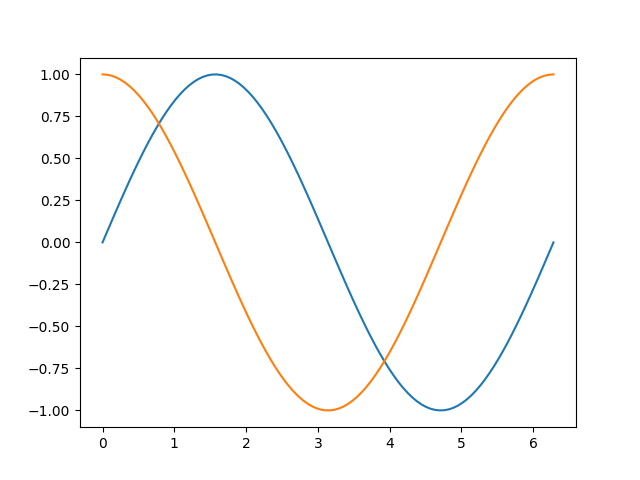
Мы использовали функцию plot, которой передали два параметра — списки значений по горизонтальной и вертикальной осям. При последовательных вызовах функции plot графики строятся в одних осях, при этом происходит автоматическое переключение цвета.
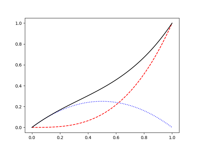
функции plot позволяет задавать тип маркера, тип линии и цвет. Приведем несколько примеров:
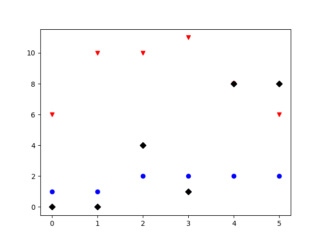
Из последнего примера видно, что если в функцию plot передать только один список y , то он будет использован для значений по вертикальной оси. В качестве значений по горизонтальной оси будет использован range(len(y)) .
Более тонкую настройку параметров можно выполнить, передавая различные именованные аргументы, например:
- marker : str — тип маркера
- markersize : float — размер маркера
- linestyle : str — тип линии
- linewidth : float — толщина линии
- color : str — цвет
Полный список доступных параметров можно найти в документации.
pyplot.errorbar
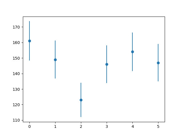
Результаты измерений в физике чаще всего представлены в виде величин с ошибками. Функция plt.errorbar позволяет отображать такие данные:
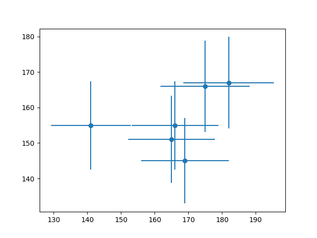
Ошибки можно задавать и для значений по горизонтальной оси:
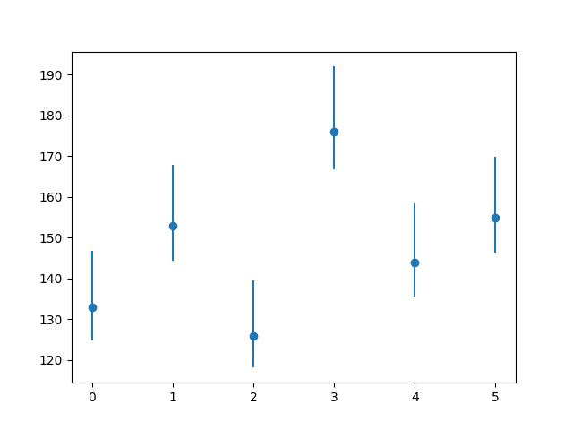
Ошибки измерений могут быть асимметричными. Для их отображения в качестве параметра yerr (или xerr ) необходимо передать кортеж из двух списков:
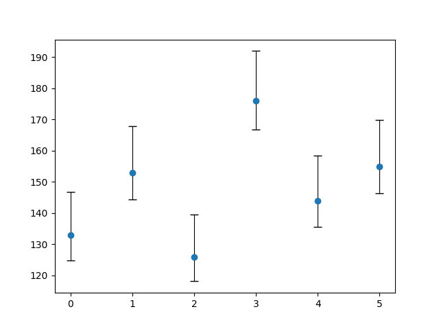
Функция pyplot.errorbar поддерживает настройку отображения графика с помощью параметра fmt и всех именованных параметров, которые доступны в функции pyplot . Кроме того, здесь появляются параметры для настройки отображения линий ошибок (“усов”):
- ecolor : str — цвет линий ошибок
- elinewidth : float — ширина линий ошибок
- capsize : float — длина “колпачков” на концах линий ошибок
- capthick : float — толщина “колпачков” на концах линий ошибок
и некоторые другие. Изменим параметры отрисовки данных из предыдущего примера:
Настройки отображения
Наши графики все еще выглядят довольно наивно. В этой части мы рассмотрим различные настройки, которые позволят достичь качества оформления диаграмм, соответствующего, например, публикациям в рецензируемых журналах.
Диапазон значений осей
Задавать диапазон значений осей в matplotlib можно несколькими способами. Например, так:
Размер шрифта
Размер и другие свойства шрифта, который используется в matplotlib по умолчанию, можно изменить с помощью объекта matplotlib.rcParams :
Объект matplotlib.rcParams хранит множество настроек, изменяя которые, можно управлять поведением по умолчанию. Смотрите подробнее в документации.
Подписи осей
Подписи к осям задаются следующим образом:
В подписях к осям (и вообще в любом тексте в matplotlib) можно использовать инструменты текстовой разметки TeX, позволяющие отрисовывать различные математические выражения. TeX-выражения должны быть внутри пары символов $ , кроме того, их следует помещать в r-строки, чтобы избежать неправильной обработки.
Заголовок
Функция pyplot.title задает заголовок диаграммы. Применим наши новые знания:
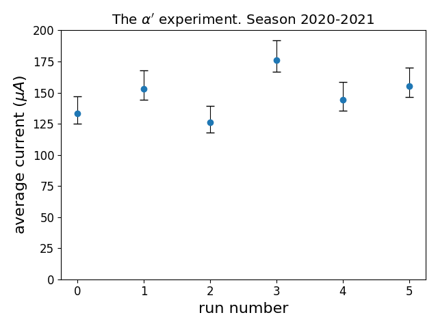
В этом примере мы использовали функцию pyplot.tight_layout, которая автоматически подбирает параметры отображения так, чтобы различные элементы не пересекались.
Легенда
При построении нескольких графиков в одних осях полезно добавлять легенду — пояснения к каждой линии. Следующий пример показывает, как это делается с помощью аргументов label и функции pyplot.legend :
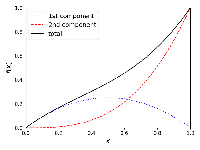
Функция pyplot.legend старается расположить легенду так, чтобы она не пересекала графики. Аргумент loc позволяет задать расположение легенды вручную. В большинстве случаев расположение по умолчанию получается удачным. Детали и описание других аргументов смотрите в документации.
Сетка
Сетка во многих случаях облегчает анализ графиков. Включить отображение сетки можно с помощью функции pyplot.grid . Аргумент axis этой функции имеет три возможных значения: x , y и both и определяет оси, вдоль которых будут проведены линии сетки. Управлять свойствами линии сетки можно с помощью именованных аргументов, которые мы рассматривали выше при обсуждении функции pyplot.plot .
В matplotlib поддерживается два типа сеток: основная и дополнительная. Выбор типа сетки выполняется с помощью аргумента which , который может принимать три значения: major , minor и both . По умолчанию используется основная сетка.
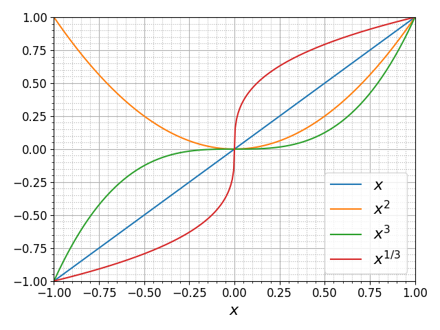
Линии сетки привязаны к отметкам на осях. Чтобы работать с дополнительной сеткой необходимо сначала включить вспомогательные отметки на осях (которые по умолчанию отключены и к которым привязаны линии дополнительной сетки) с помощью функции pyplot.minorticks_on . Приведем пример:
Логарифмический масштаб
Функции pyplot.semilogy и pyplot.semilogx выполняют переключение между линейным и логарифмическим масштабами осей. В некоторых случаях логарифмический масштаб позволяет отобразить особенности зависимостей, которые не видны в линейном масштабе. Вот так выглядят графики экспоненциальных функций в линейном масштабе:
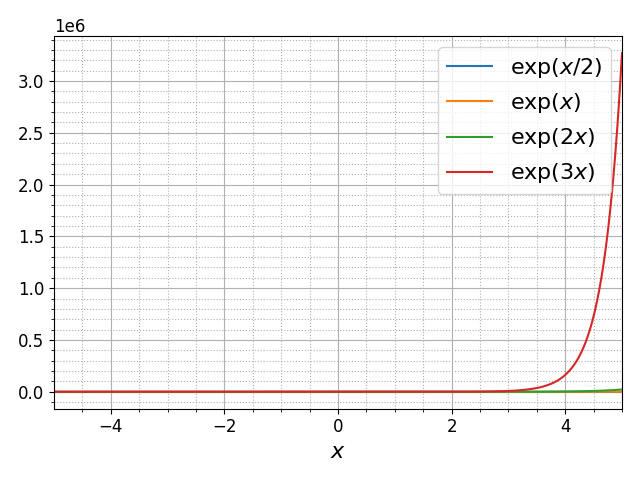
делает график гораздо более информативным:
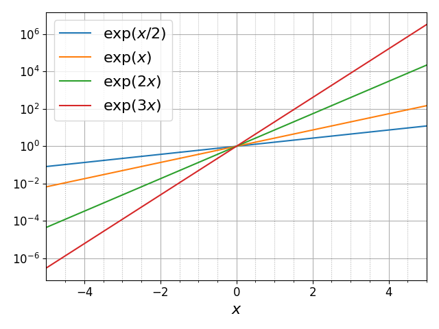
Теперь мы видим поведение функций во всем динамическом диапазоне, занимающем 12 порядков.
Произвольные отметки на осях
Вернемся к первому примеру, в котором мы строили графики синуса и косинуса. Сделаем так, чтобы на горизонтальной оси отметки соответствовали различным долям числа pi и имели соответствующие подписи:
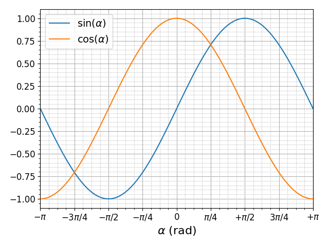
Метки на горизонтальной оси были заданы с помощью функции pyplot.xticks :
Модуль pyplot.ticker содержит более продвинутые инструменты для управления отметками на осях. Подробности смотрите в документации.
Размер изображения
До сих пор мы строили графики в одном окне, размер которого был задан по умолчанию. За кадром matplotlib создавал объект типа Figure, который определяет размер окна и содержит все остальные элементы. Кроме того, автоматически создавался объект типа Axis. Подробнее работа с этими объектами будет рассмотрена ниже. Сейчас же мы рассмотрим функцию pyplot.figure , которая позволяет создавать новые объекты типа Figure и переключаться между уже созданными объектами.
Функция pyplot.figure может принимать множество аргументов. Вот основные:
- num : int или str — уникальный идентификатор объекта типа. Если задан новый идентификатор, то создается новый объект и он становится активным. В случае, если передан идентификатор уже существующего объекта, то этот объект возвращается и становится активным
- figsize : (float, float) — размер изображения в дюймах
- dpi : float — разрешение в количестве точек на дюйм
Описание других параметров функции pyplot.figure можно найти в документации. Используем эту функцию и функцию pyplot.axis чтобы улучшить наш пример с построением степенных функций:
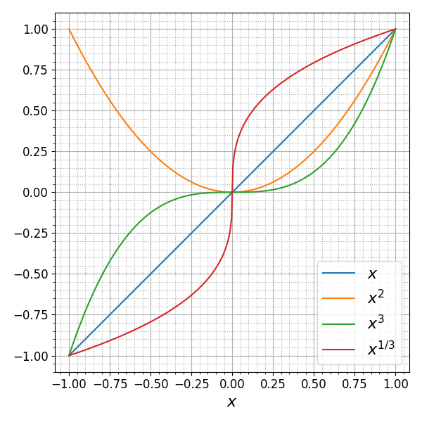
Мы добавили две строки по сравнению с прошлой версией:
Функция pyplot.axis позволяет задавать некоторые свойства осей. Ее вызов с параметром ‘equal’ делает одинаковыми масштабы вертикальной и горизонтальной осей, что кажется хорошей идеей в этом примере. Функция pyplot.axis возвращает кортеж из четырех значений xmin, xmax, ymin, ymax , соответствующих границам диапазонов значений осей.
Некоторые другие способы использования функции pyplot.axis :
- Кортеж из четырех float задаст новые границы диапазонов значений осей
- Строка ‘off’ выключит отображение линий и меток осей
Гистограммы
Обратимся теперь к другим типам диаграмм. Функция pyplot.hist строит гистограмму по набору значений:
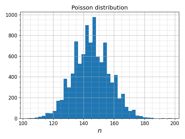
Аргумент bins задает количество бинов гистограммы. По умолчанию используется значение 10. Если вместо целого числа в аргумент bins передать кортеж значений, то они будут использованы для задания границ бинов. Таким образом можно построить гистограмму с произвольным разбиением.
Некоторые другие аргументы функции pyplot.hist :
- range : (float, float) — диапазон значений, в котором строится гистограмма. Значения за пределами заданного диапазона игнорируются.
- density : bool . При значении True будет построена гистограмма, соответствующая плотности вероятности, так что площадь гистограммы будет равна единице.
- weights : список float значений того же размера, что и набор данных. Определяет вес каждого значения при построении гистограммы.
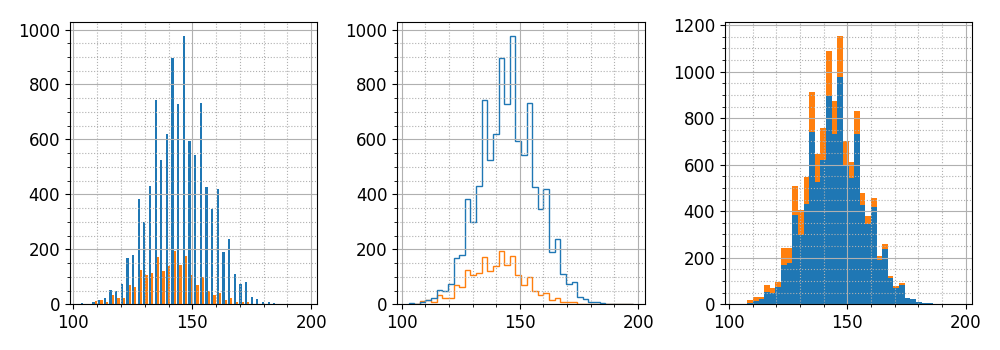
- histtype : str . может принимать значения <'bar', 'barstacked', 'step', 'stepfilled'>. Определяет тип отрисовки гистограммы.
В качестве первого аргумента можно передать кортеж наборов значений. Для каждого из них будет построена гистограмма. Аргумент stacked со значением True позволяет строить сумму гистограмм для кортежа наборов. Покажем несколько примеров:
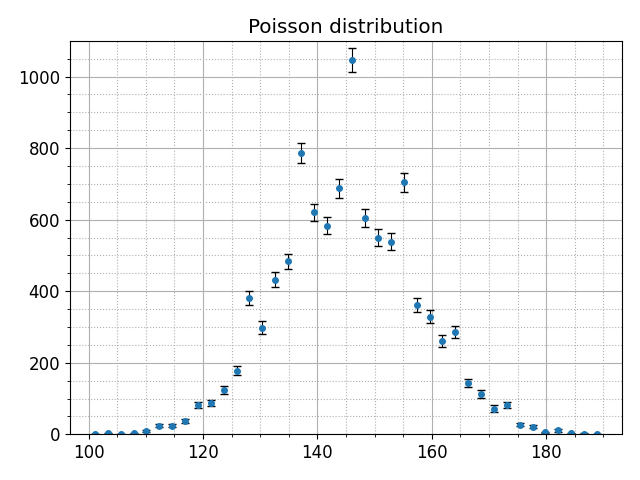
В физике гистограммы часто представляют в виде набора значений с ошибками, предполагая при этом, что количество событий в каждом бине является случайной величиной, подчиняющейся биномиальному распределению. В пределе больших значений флуктуации количества событий в бине могут быть описаны распределением Пуассона, так что характерная величина флуктуации определяется корнем из числа событий. Библиотека matplotlib не имеет инструмента для такого представления данных, однако его легко получить с помощью комбинации numpy.histogram и pyplot.errorbar :
Диаграммы рассеяния
Распределение событий по двум измерениям удобно визуализировать с помощью диаграммы рассеяния:
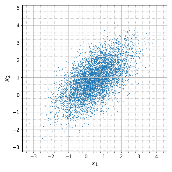
Каждой паре значений в наборе данных соответствует одна точка на диаграмме. Несмотря на свою простоту, диаграмма рассеяния позволяет во многих случаях наглядно представлять двумерные данные. Функция pyplot.scatter позволяет визуализировать и данные более высокой размерности: размер и цвет маркера могут быть заданы для каждой точки отдельно:
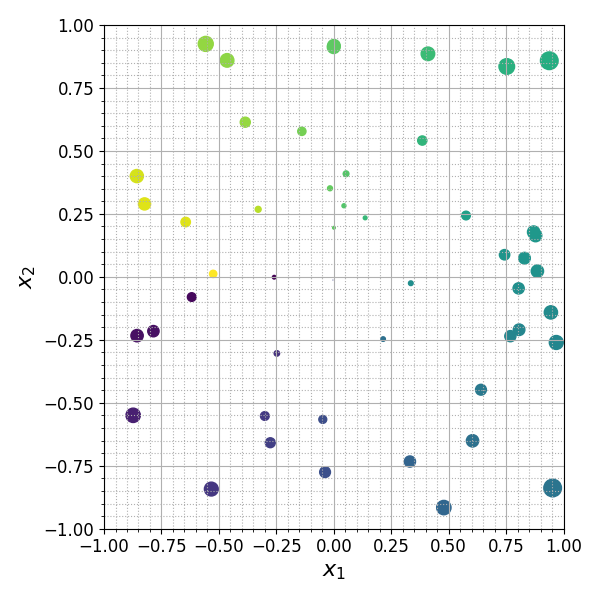
Цветовую палитру можно задать с помощью аргумента cmap . Подробности и описание других аргументов функции pyplot.scatter можно найти в документации.
Контурные диаграммы
Контурные диаграммы позволяют визуализировать функции двух переменных:
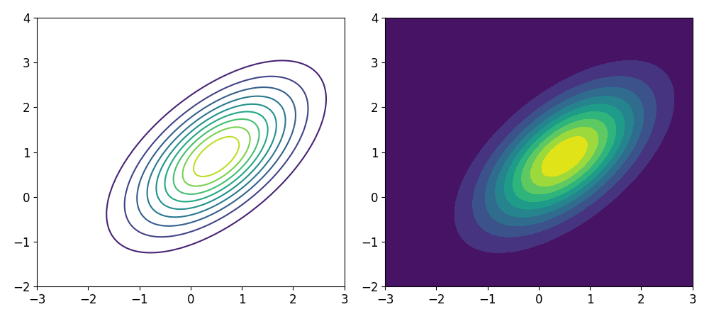
Аргумент levels задает количество контуров. По умолчанию контуры отрисовываются равномерно между максимальным и минимальным значениями. В аргумент levels также можно передать список уровней, на которых следует провести контуры.
Обратите внимание на использование функций numpy.meshgrid и numpy.dstack в этом примере.
Контурную диаграмму можно дополнить цветовой полосой colorbar , вызвав функцию pyplot.colorbar :
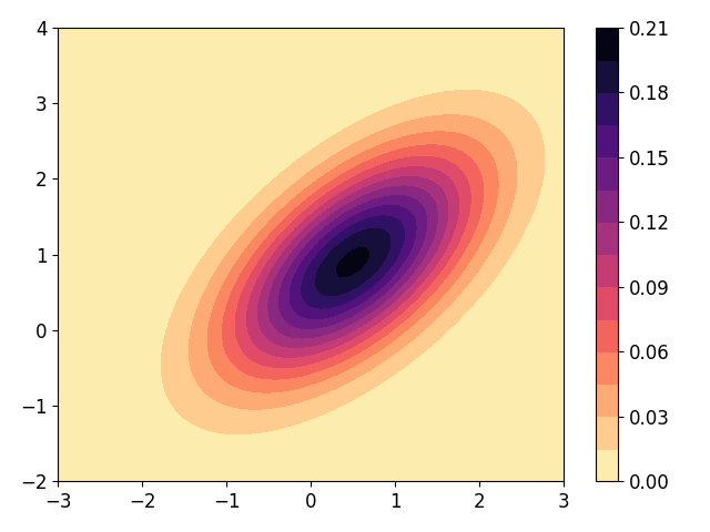
Более подробное описание функций plt.contour и plt.contourf смотрите в документации.
Расположение нескольких осей в одном окне
В одном окне (объекте Figure ) можно разместить несколько осей (объектов axis.Axis ). Функция pyplot.subplots создает объект Figure , содержащий регулярную сетку объектов axis.Axis :
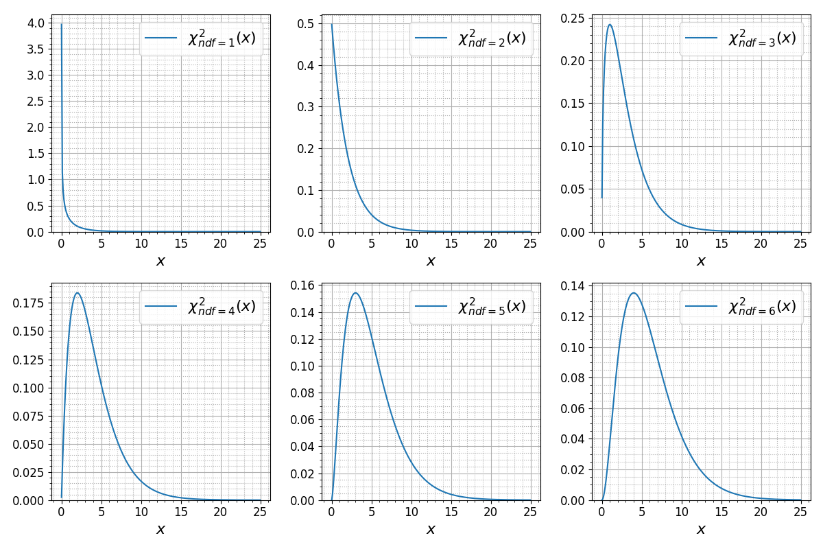
Количество строк и столбцов, по которым располагаются различные оси, задаются с помощью параметров nrows и ncols , соответственно. Функция pyplot.subplots возвращает объект Figure и двумерный список осей axis.Axis . Обратите внимание на то, что вместо вызовов функций модуля pyplot в этом примере использовались вызовы методов классов Figure и axis.Axis .
В последнем примере горизонтальная ось во всех графиках имеет один и тот же диапазон. Аргумент sharex функции pyplot.subplots позволяет убрать дублирование отрисовки осей в таких случаях:
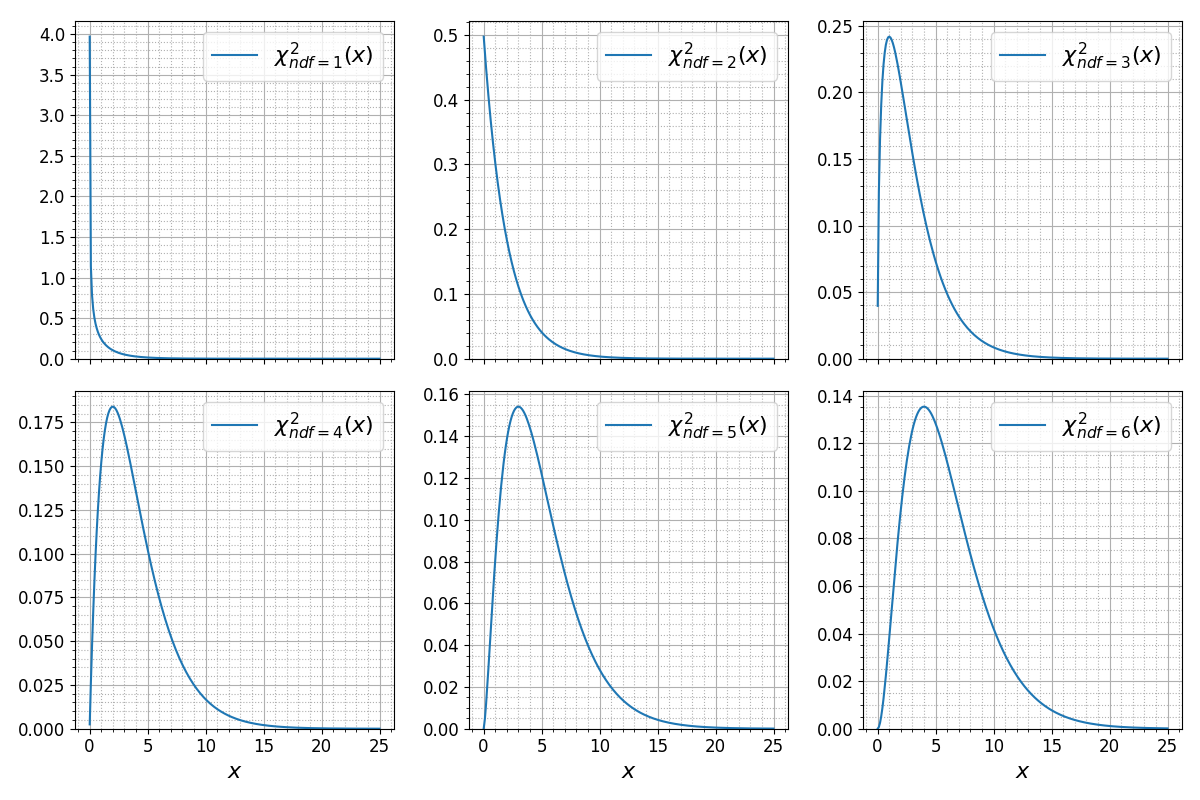
Существует аналогичный параметр sharey для вертикальной оси.
Более гибкие возможности регулярного расположения осей предоставляет функция pyplot.subplot. Мы не будем рассматривать эту функцию и ограничимся лишь ее упоминанием.
Функция pyplot.axes позволяет добавлять новые оси в текущем окне в произвольном месте:
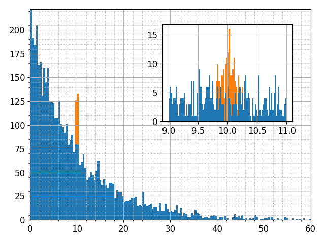
В этом примере была использована функция pyplot.savefig , сохраняющая содержимое текущего окна в файл в векторном или растровом формате. Формат задается с помощью аргумента format или автоматически определяется из имени файла (как в примере выше). Набор доступных форматов зависит от окружения, однако в большинстве случаев можно использовать такие форматы как png , jpeg , pdf , svg и eps .
Резюме
Предметом изучения в этом разделе был модуль pyplot библиотеки matplotlib , содержащий инструменты для построения различных диаграмм. Были рассмотрены:
- функции для построения диаграмм pyplot.plot , pyplot.errorbar . pyplot.hist , pyplot.scatter , pyplot.contour и pyplot.contourf ;
- средства настройки свойств линий и маркеров;
- средства настройки координатных осей: подписи, размер шрифта, координатная сетка, произвольные метки др.;
- инструмены для расположения нескольких координатных осей в одном окне.
Рассмотренные инструменты далеко не исчерпывают возможности библиотеки matplotlib , однако их должно быть достаточно в большинстве случаев для визуализации данных. Мы рекомендуем заинтересованному читалелю изучить список источников, в которых можно найти много дополнительной информации.