Как выбрать строки по индексу в Pandas DataFrame
Часто вам может понадобиться выбрать строки кадра данных pandas на основе их значения индекса.
Если вы хотите выбрать строки на основе целочисленного индексирования, вы можете использовать функцию .iloc .
Если вы хотите выбрать строки на основе индексации меток, вы можете использовать функцию .loc .
В этом руководстве представлен пример использования каждой из этих функций на практике.
Пример 1: выбор строк на основе целочисленного индексирования
В следующем коде показано, как создать кадр данных pandas и использовать .iloc для выбора строки с целочисленным значением индекса 4 :
Мы можем использовать аналогичный синтаксис для выбора нескольких строк:
Или мы могли бы выбрать все строки в диапазоне:
Пример 2. Выбор строк на основе индексации меток
В следующем коде показано, как создать кадр данных pandas и использовать .loc для выбора строки с меткой индекса 3 :
Мы можем использовать аналогичный синтаксис для выбора нескольких строк с разными метками индекса:
Разница между .iloc и .loc
Приведенные выше примеры иллюстрируют тонкую разницу между .iloc и .loc :
Indexing and selecting data#
The axis labeling information in pandas objects serves many purposes:
Identifies data (i.e. provides metadata) using known indicators, important for analysis, visualization, and interactive console display.
Enables automatic and explicit data alignment.
Allows intuitive getting and setting of subsets of the data set.
In this section, we will focus on the final point: namely, how to slice, dice, and generally get and set subsets of pandas objects. The primary focus will be on Series and DataFrame as they have received more development attention in this area.
The Python and NumPy indexing operators [] and attribute operator . provide quick and easy access to pandas data structures across a wide range of use cases. This makes interactive work intuitive, as there’s little new to learn if you already know how to deal with Python dictionaries and NumPy arrays. However, since the type of the data to be accessed isn’t known in advance, directly using standard operators has some optimization limits. For production code, we recommended that you take advantage of the optimized pandas data access methods exposed in this chapter.
Whether a copy or a reference is returned for a setting operation, may depend on the context. This is sometimes called chained assignment and should be avoided. See Returning a View versus Copy .
See the MultiIndex / Advanced Indexing for MultiIndex and more advanced indexing documentation.
See the cookbook for some advanced strategies.
Different choices for indexing#
Object selection has had a number of user-requested additions in order to support more explicit location based indexing. pandas now supports three types of multi-axis indexing.
.loc is primarily label based, but may also be used with a boolean array. .loc will raise KeyError when the items are not found. Allowed inputs are:
-
A single label, e.g. 5 or ‘a’ (Note that 5 is interpreted as a label of the index. This use is not an integer position along the index.).
-
A list or array of labels [‘a’, ‘b’, ‘c’] .
-
A slice object with labels ‘a’:’f’ (Note that contrary to usual Python slices, both the start and the stop are included, when present in the index! See Slicing with labels and Endpoints are inclusive .)
-
A boolean array (any NA values will be treated as False ).
-
A callable function with one argument (the calling Series or DataFrame) and that returns valid output for indexing (one of the above).
.iloc is primarily integer position based (from 0 to length-1 of the axis), but may also be used with a boolean array. .iloc will raise IndexError if a requested indexer is out-of-bounds, except slice indexers which allow out-of-bounds indexing. (this conforms with Python/NumPy slice semantics). Allowed inputs are:
-
An integer e.g. 5 .
-
A list or array of integers [4, 3, 0] .
-
A slice object with ints 1:7 .
-
A boolean array (any NA values will be treated as False ).
-
A callable function with one argument (the calling Series or DataFrame) and that returns valid output for indexing (one of the above).
.loc , .iloc , and also [] indexing can accept a callable as indexer. See more at Selection By Callable .
Getting values from an object with multi-axes selection uses the following notation (using .loc as an example, but the following applies to .iloc as well). Any of the axes accessors may be the null slice : . Axes left out of the specification are assumed to be : , e.g. p.loc[‘a’] is equivalent to p.loc[‘a’, :] .
Basics#
As mentioned when introducing the data structures in the last section , the primary function of indexing with [] (a.k.a. __getitem__ for those familiar with implementing class behavior in Python) is selecting out lower-dimensional slices. The following table shows return type values when indexing pandas objects with [] :
Return Value Type
Series corresponding to colname
Here we construct a simple time series data set to use for illustrating the indexing functionality:
None of the indexing functionality is time series specific unless specifically stated.
Thus, as per above, we have the most basic indexing using [] :
You can pass a list of columns to [] to select columns in that order. If a column is not contained in the DataFrame, an exception will be raised. Multiple columns can also be set in this manner:
You may find this useful for applying a transform (in-place) to a subset of the columns.
pandas aligns all AXES when setting Series and DataFrame from .loc , and .iloc .
This will not modify df because the column alignment is before value assignment.
The correct way to swap column values is by using raw values:
Attribute access#
You may access an index on a Series or column on a DataFrame directly as an attribute:
You can use this access only if the index element is a valid Python identifier, e.g. s.1 is not allowed. See here for an explanation of valid identifiers.
The attribute will not be available if it conflicts with an existing method name, e.g. s.min is not allowed, but s[‘min’] is possible.
Similarly, the attribute will not be available if it conflicts with any of the following list: index , major_axis , minor_axis , items .
In any of these cases, standard indexing will still work, e.g. s[‘1’] , s[‘min’] , and s[‘index’] will access the corresponding element or column.
If you are using the IPython environment, you may also use tab-completion to see these accessible attributes.
You can also assign a dict to a row of a DataFrame :
You can use attribute access to modify an existing element of a Series or column of a DataFrame, but be careful; if you try to use attribute access to create a new column, it creates a new attribute rather than a new column and will this raise a UserWarning :
Slicing ranges#
The most robust and consistent way of slicing ranges along arbitrary axes is described in the Selection by Position section detailing the .iloc method. For now, we explain the semantics of slicing using the [] operator.
With Series, the syntax works exactly as with an ndarray, returning a slice of the values and the corresponding labels:
Note that setting works as well:
With DataFrame, slicing inside of [] slices the rows. This is provided largely as a convenience since it is such a common operation.
Selection by label#
Whether a copy or a reference is returned for a setting operation, may depend on the context. This is sometimes called chained assignment and should be avoided. See Returning a View versus Copy .
.loc is strict when you present slicers that are not compatible (or convertible) with the index type. For example using integers in a DatetimeIndex . These will raise a TypeError .
String likes in slicing can be convertible to the type of the index and lead to natural slicing.
pandas provides a suite of methods in order to have purely label based indexing. This is a strict inclusion based protocol. Every label asked for must be in the index, or a KeyError will be raised. When slicing, both the start bound AND the stop bound are included, if present in the index. Integers are valid labels, but they refer to the label and not the position.
The .loc attribute is the primary access method. The following are valid inputs:
A single label, e.g. 5 or ‘a’ (Note that 5 is interpreted as a label of the index. This use is not an integer position along the index.).
A list or array of labels [‘a’, ‘b’, ‘c’] .
A slice object with labels ‘a’:’f’ (Note that contrary to usual Python slices, both the start and the stop are included, when present in the index! See Slicing with labels .
A boolean array.
Note that setting works as well:
With a DataFrame:
Accessing via label slices:
For getting a cross section using a label (equivalent to df.xs(‘a’) ):
For getting values with a boolean array:
NA values in a boolean array propagate as False :
Changed in version 1.0.2.
For getting a value explicitly:
Slicing with labels#
When using .loc with slices, if both the start and the stop labels are present in the index, then elements located between the two (including them) are returned:
If at least one of the two is absent, but the index is sorted, and can be compared against start and stop labels, then slicing will still work as expected, by selecting labels which rank between the two:
However, if at least one of the two is absent and the index is not sorted, an error will be raised (since doing otherwise would be computationally expensive, as well as potentially ambiguous for mixed type indexes). For instance, in the above example, s.loc[1:6] would raise KeyError .
For the rationale behind this behavior, see Endpoints are inclusive .
Also, if the index has duplicate labels and either the start or the stop label is duplicated, an error will be raised. For instance, in the above example, s.loc[2:5] would raise a KeyError .
For more information about duplicate labels, see Duplicate Labels .
Selection by position#
Whether a copy or a reference is returned for a setting operation, may depend on the context. This is sometimes called chained assignment and should be avoided. See Returning a View versus Copy .
pandas provides a suite of methods in order to get purely integer based indexing. The semantics follow closely Python and NumPy slicing. These are 0-based indexing. When slicing, the start bound is included, while the upper bound is excluded. Trying to use a non-integer, even a valid label will raise an IndexError .
The .iloc attribute is the primary access method. The following are valid inputs:
An integer e.g. 5 .
A list or array of integers [4, 3, 0] .
A slice object with ints 1:7 .
A boolean array.
Note that setting works as well:
With a DataFrame:
Select via integer slicing:
Select via integer list:
For getting a cross section using an integer position (equiv to df.xs(1) ):
Out of range slice indexes are handled gracefully just as in Python/NumPy.
Note that using slices that go out of bounds can result in an empty axis (e.g. an empty DataFrame being returned).
A single indexer that is out of bounds will raise an IndexError . A list of indexers where any element is out of bounds will raise an IndexError .
Selection by callable#
.loc , .iloc , and also [] indexing can accept a callable as indexer. The callable must be a function with one argument (the calling Series or DataFrame) that returns valid output for indexing.
You can use callable indexing in Series .
Using these methods / indexers, you can chain data selection operations without using a temporary variable.
Combining positional and label-based indexing#
If you wish to get the 0th and the 2nd elements from the index in the ‘A’ column, you can do:
This can also be expressed using .iloc , by explicitly getting locations on the indexers, and using positional indexing to select things.
For getting multiple indexers, using .get_indexer :
Indexing with list with missing labels is deprecated#
In prior versions, using .loc[list-of-labels] would work as long as at least 1 of the keys was found (otherwise it would raise a KeyError ). This behavior was changed and will now raise a KeyError if at least one label is missing. The recommended alternative is to use .reindex() .
Selection with all keys found is unchanged.
Reindexing#
The idiomatic way to achieve selecting potentially not-found elements is via .reindex() . See also the section on reindexing .
Alternatively, if you want to select only valid keys, the following is idiomatic and efficient; it is guaranteed to preserve the dtype of the selection.
Having a duplicated index will raise for a .reindex() :
Generally, you can intersect the desired labels with the current axis, and then reindex.
However, this would still raise if your resulting index is duplicated.
Selecting random samples#
A random selection of rows or columns from a Series or DataFrame with the sample() method. The method will sample rows by default, and accepts a specific number of rows/columns to return, or a fraction of rows.
By default, sample will return each row at most once, but one can also sample with replacement using the replace option:
By default, each row has an equal probability of being selected, but if you want rows to have different probabilities, you can pass the sample function sampling weights as weights . These weights can be a list, a NumPy array, or a Series, but they must be of the same length as the object you are sampling. Missing values will be treated as a weight of zero, and inf values are not allowed. If weights do not sum to 1, they will be re-normalized by dividing all weights by the sum of the weights. For example:
When applied to a DataFrame, you can use a column of the DataFrame as sampling weights (provided you are sampling rows and not columns) by simply passing the name of the column as a string.
sample also allows users to sample columns instead of rows using the axis argument.
Finally, one can also set a seed for sample ’s random number generator using the random_state argument, which will accept either an integer (as a seed) or a NumPy RandomState object.
Setting with enlargement#
The .loc/[] operations can perform enlargement when setting a non-existent key for that axis.
In the Series case this is effectively an appending operation.
A DataFrame can be enlarged on either axis via .loc .
This is like an append operation on the DataFrame .
Fast scalar value getting and setting#
Since indexing with [] must handle a lot of cases (single-label access, slicing, boolean indexing, etc.), it has a bit of overhead in order to figure out what you’re asking for. If you only want to access a scalar value, the fastest way is to use the at and iat methods, which are implemented on all of the data structures.
Similarly to loc , at provides label based scalar lookups, while, iat provides integer based lookups analogously to iloc
You can also set using these same indexers.
at may enlarge the object in-place as above if the indexer is missing.
Boolean indexing#
Another common operation is the use of boolean vectors to filter the data. The operators are: | for or , & for and , and
for not . These must be grouped by using parentheses, since by default Python will evaluate an expression such as df[‘A’] > 2 & df[‘B’] < 3 as df[‘A’] > (2 & df[‘B’]) < 3 , while the desired evaluation order is (df[‘A’] > 2) & (df[‘B’] < 3) .
Using a boolean vector to index a Series works exactly as in a NumPy ndarray:
You may select rows from a DataFrame using a boolean vector the same length as the DataFrame’s index (for example, something derived from one of the columns of the DataFrame):
List comprehensions and the map method of Series can also be used to produce more complex criteria:
With the choice methods Selection by Label , Selection by Position , and Advanced Indexing you may select along more than one axis using boolean vectors combined with other indexing expressions.
iloc supports two kinds of boolean indexing. If the indexer is a boolean Series , an error will be raised. For instance, in the following example, df.iloc[s.values, 1] is ok. The boolean indexer is an array. But df.iloc[s, 1] would raise ValueError .
Indexing with isin#
Consider the isin() method of Series , which returns a boolean vector that is true wherever the Series elements exist in the passed list. This allows you to select rows where one or more columns have values you want:
The same method is available for Index objects and is useful for the cases when you don’t know which of the sought labels are in fact present:
In addition to that, MultiIndex allows selecting a separate level to use in the membership check:
DataFrame also has an isin() method. When calling isin , pass a set of values as either an array or dict. If values is an array, isin returns a DataFrame of booleans that is the same shape as the original DataFrame, with True wherever the element is in the sequence of values.
Oftentimes you’ll want to match certain values with certain columns. Just make values a dict where the key is the column, and the value is a list of items you want to check for.
To return the DataFrame of booleans where the values are not in the original DataFrame, use the
Combine DataFrame’s isin with the any() and all() methods to quickly select subsets of your data that meet a given criteria. To select a row where each column meets its own criterion:
The where() Method and Masking#
Selecting values from a Series with a boolean vector generally returns a subset of the data. To guarantee that selection output has the same shape as the original data, you can use the where method in Series and DataFrame .
To return only the selected rows:
To return a Series of the same shape as the original:
Selecting values from a DataFrame with a boolean criterion now also preserves input data shape. where is used under the hood as the implementation. The code below is equivalent to df.where(df < 0) .
In addition, where takes an optional other argument for replacement of values where the condition is False, in the returned copy.
You may wish to set values based on some boolean criteria. This can be done intuitively like so:
where returns a modified copy of the data.
The signature for DataFrame.where() differs from numpy.where() . Roughly df1.where(m, df2) is equivalent to np.where(m, df1, df2) .
Alignment
Furthermore, where aligns the input boolean condition (ndarray or DataFrame), such that partial selection with setting is possible. This is analogous to partial setting via .loc (but on the contents rather than the axis labels).
Where can also accept axis and level parameters to align the input when performing the where .
This is equivalent to (but faster than) the following.
where can accept a callable as condition and other arguments. The function must be with one argument (the calling Series or DataFrame) and that returns valid output as condition and other argument.
mask() is the inverse boolean operation of where .
Setting with enlargement conditionally using numpy() #
An alternative to where() is to use numpy.where() . Combined with setting a new column, you can use it to enlarge a DataFrame where the values are determined conditionally.
Consider you have two choices to choose from in the following DataFrame. And you want to set a new column color to ‘green’ when the second column has ‘Z’. You can do the following:
If you have multiple conditions, you can use numpy.select() to achieve that. Say corresponding to three conditions there are three choice of colors, with a fourth color as a fallback, you can do the following.
The query() Method#
DataFrame objects have a query() method that allows selection using an expression.
You can get the value of the frame where column b has values between the values of columns a and c . For example:
Do the same thing but fall back on a named index if there is no column with the name a .
If instead you don’t want to or cannot name your index, you can use the name index in your query expression:
If the name of your index overlaps with a column name, the column name is given precedence. For example,
You can still use the index in a query expression by using the special identifier ‘index’:
If for some reason you have a column named index , then you can refer to the index as ilevel_0 as well, but at this point you should consider renaming your columns to something less ambiguous.
MultiIndex query() Syntax#
You can also use the levels of a DataFrame with a MultiIndex as if they were columns in the frame:
If the levels of the MultiIndex are unnamed, you can refer to them using special names:
The convention is ilevel_0 , which means “index level 0” for the 0th level of the index .
query() Use Cases#
A use case for query() is when you have a collection of DataFrame objects that have a subset of column names (or index levels/names) in common. You can pass the same query to both frames without having to specify which frame you’re interested in querying
query() Python versus pandas Syntax Comparison#
Full numpy-like syntax:
Slightly nicer by removing the parentheses (comparison operators bind tighter than & and | ):
Use English instead of symbols:
Pretty close to how you might write it on paper:
The in and not in operators#
query() also supports special use of Python’s in and not in comparison operators, providing a succinct syntax for calling the isin method of a Series or DataFrame .
You can combine this with other expressions for very succinct queries:
Note that in and not in are evaluated in Python, since numexpr has no equivalent of this operation. However, only the in / not in expression itself is evaluated in vanilla Python. For example, in the expression
(b + c + d) is evaluated by numexpr and then the in operation is evaluated in plain Python. In general, any operations that can be evaluated using numexpr will be.
Special use of the == operator with list objects#
Comparing a list of values to a column using == / != works similarly to in / not in .
Boolean operators#
You can negate boolean expressions with the word not or the
Of course, expressions can be arbitrarily complex too:
Performance of query() #
DataFrame.query() using numexpr is slightly faster than Python for large frames.
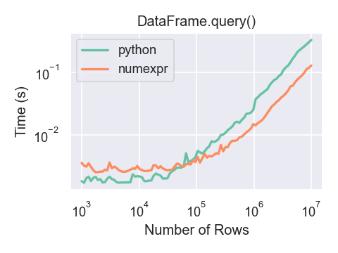
You will only see the performance benefits of using the numexpr engine with DataFrame.query() if your frame has more than approximately 100,000 rows.
This plot was created using a DataFrame with 3 columns each containing floating point values generated using numpy.random.randn() .
Duplicate data#
If you want to identify and remove duplicate rows in a DataFrame, there are two methods that will help: duplicated and drop_duplicates . Each takes as an argument the columns to use to identify duplicated rows.
duplicated returns a boolean vector whose length is the number of rows, and which indicates whether a row is duplicated.
drop_duplicates removes duplicate rows.
By default, the first observed row of a duplicate set is considered unique, but each method has a keep parameter to specify targets to be kept.
keep=’first’ (default): mark / drop duplicates except for the first occurrence.
keep=’last’ : mark / drop duplicates except for the last occurrence.
keep=False : mark / drop all duplicates.
Also, you can pass a list of columns to identify duplications.
To drop duplicates by index value, use Index.duplicated then perform slicing. The same set of options are available for the keep parameter.
Dictionary-like get() method#
Each of Series or DataFrame have a get method which can return a default value.
Looking up values by index/column labels#
Sometimes you want to extract a set of values given a sequence of row labels and column labels, this can be achieved by pandas.factorize and NumPy indexing. For instance:
Formerly this could be achieved with the dedicated DataFrame.lookup method which was deprecated in version 1.2.0 and removed in version 2.0.0.
Index objects#
The pandas Index class and its subclasses can be viewed as implementing an ordered multiset. Duplicates are allowed. However, if you try to convert an Index object with duplicate entries into a set , an exception will be raised.
Index also provides the infrastructure necessary for lookups, data alignment, and reindexing. The easiest way to create an Index directly is to pass a list or other sequence to Index :
or using numbers:
If no dtype is given, Index tries to infer the dtype from the data. It is also possible to give an explicit dtype when instantiating an Index :
You can also pass a name to be stored in the index:
The name, if set, will be shown in the console display:
Setting metadata#
Indexes are “mostly immutable”, but it is possible to set and change their name attribute. You can use the rename , set_names to set these attributes directly, and they default to returning a copy.
See Advanced Indexing for usage of MultiIndexes.
set_names , set_levels , and set_codes also take an optional level argument
Set operations on Index objects#
The two main operations are union and intersection . Difference is provided via the .difference() method.
Also available is the symmetric_difference operation, which returns elements that appear in either idx1 or idx2 , but not in both. This is equivalent to the Index created by idx1.difference(idx2).union(idx2.difference(idx1)) , with duplicates dropped.
The resulting index from a set operation will be sorted in ascending order.
When performing Index.union() between indexes with different dtypes, the indexes must be cast to a common dtype. Typically, though not always, this is object dtype. The exception is when performing a union between integer and float data. In this case, the integer values are converted to float
Missing values#
Even though Index can hold missing values ( NaN ), it should be avoided if you do not want any unexpected results. For example, some operations exclude missing values implicitly.
Index.fillna fills missing values with specified scalar value.
Set / reset index#
Occasionally you will load or create a data set into a DataFrame and want to add an index after you’ve already done so. There are a couple of different ways.
Set an index#
DataFrame has a set_index() method which takes a column name (for a regular Index ) or a list of column names (for a MultiIndex ). To create a new, re-indexed DataFrame:
The append keyword option allow you to keep the existing index and append the given columns to a MultiIndex:
Other options in set_index allow you not drop the index columns.
Reset the index#
As a convenience, there is a new function on DataFrame called reset_index() which transfers the index values into the DataFrame’s columns and sets a simple integer index. This is the inverse operation of set_index() .
The output is more similar to a SQL table or a record array. The names for the columns derived from the index are the ones stored in the names attribute.
You can use the level keyword to remove only a portion of the index:
reset_index takes an optional parameter drop which if true simply discards the index, instead of putting index values in the DataFrame’s columns.
Adding an ad hoc index#
If you create an index yourself, you can just assign it to the index field:
Returning a view versus a copy#
When setting values in a pandas object, care must be taken to avoid what is called chained indexing . Here is an example.
Compare these two access methods:
These both yield the same results, so which should you use? It is instructive to understand the order of operations on these and why method 2 ( .loc ) is much preferred over method 1 (chained [] ).
dfmi[‘one’] selects the first level of the columns and returns a DataFrame that is singly-indexed. Then another Python operation dfmi_with_one[‘second’] selects the series indexed by ‘second’ . This is indicated by the variable dfmi_with_one because pandas sees these operations as separate events. e.g. separate calls to __getitem__ , so it has to treat them as linear operations, they happen one after another.
Contrast this to df.loc[:,(‘one’,’second’)] which passes a nested tuple of (slice(None),(‘one’,’second’)) to a single call to __getitem__ . This allows pandas to deal with this as a single entity. Furthermore this order of operations can be significantly faster, and allows one to index both axes if so desired.
Why does assignment fail when using chained indexing?#
The problem in the previous section is just a performance issue. What’s up with the SettingWithCopy warning? We don’t usually throw warnings around when you do something that might cost a few extra milliseconds!
But it turns out that assigning to the product of chained indexing has inherently unpredictable results. To see this, think about how the Python interpreter executes this code:
But this code is handled differently:
See that __getitem__ in there? Outside of simple cases, it’s very hard to predict whether it will return a view or a copy (it depends on the memory layout of the array, about which pandas makes no guarantees), and therefore whether the __setitem__ will modify dfmi or a temporary object that gets thrown out immediately afterward. That’s what SettingWithCopy is warning you about!
You may be wondering whether we should be concerned about the loc property in the first example. But dfmi.loc is guaranteed to be dfmi itself with modified indexing behavior, so dfmi.loc.__getitem__ / dfmi.loc.__setitem__ operate on dfmi directly. Of course, dfmi.loc.__getitem__(idx) may be a view or a copy of dfmi .
Sometimes a SettingWithCopy warning will arise at times when there’s no obvious chained indexing going on. These are the bugs that SettingWithCopy is designed to catch! pandas is probably trying to warn you that you’ve done this:
Evaluation order matters#
When you use chained indexing, the order and type of the indexing operation partially determine whether the result is a slice into the original object, or a copy of the slice.
pandas has the SettingWithCopyWarning because assigning to a copy of a slice is frequently not intentional, but a mistake caused by chained indexing returning a copy where a slice was expected.
If you would like pandas to be more or less trusting about assignment to a chained indexing expression, you can set the option mode.chained_assignment to one of these values:
‘warn’ , the default, means a SettingWithCopyWarning is printed.
‘raise’ means pandas will raise a SettingWithCopyError you have to deal with.
None will suppress the warnings entirely.
This however is operating on a copy and will not work.
A chained assignment can also crop up in setting in a mixed dtype frame.
These setting rules apply to all of .loc/.iloc .
The following is the recommended access method using .loc for multiple items (using mask ) and a single item using a fixed index:
The following can work at times, but it is not guaranteed to, and therefore should be avoided:
Last, the subsequent example will not work at all, and so should be avoided:
The chained assignment warnings / exceptions are aiming to inform the user of a possibly invalid assignment. There may be false positives; situations where a chained assignment is inadvertently reported.
Доступ по индексу в DataFrame
Мы уже рассказывали о структуре DataFrame в Pandas — высокоуровневой Python-библиотеке для анализа данных. Но как осуществляется доступ по индексу в DataFrame?
На самом деле, индекс по строкам мы можем задавать различными способами, к примеру, в процессе формирования самого объекта DataFrame либо, как говорится «на лету»:
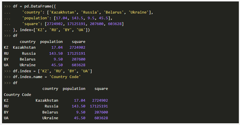
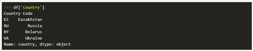
Таким образом, мы видим, что индексу задается имя Country Code. Также стоит отметить, что объекты Series из DataFrame приобретут те же самые индексы, что и объект DataFrame:
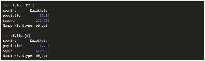
При этом доступ к строкам по индексу можно осуществить 2-мя способами:
- .loc — для доступа по строковой метке;
- .iloc — для доступа по числовому значению (от 0 и выше).
Идем дальше. У нас есть возможность выполнять выборку по индексу и интересующим колонкам:

Обратите внимание, что .loc в квадратных скобках принимает два аргумента. Кроме интересующего индекса, поддерживаются колонки и слайсинг.

Следующий момент — у нас есть возможность фильтровать DataFrame, используя для этого булевы массивы:

Кроме того, существует возможность обращения к столбцам — для этого применяется атрибут либо нотация словарей Python, то есть df.population и df[‘population’] — это, по сути, одно и то же.
Если надо сбросить индексы, сделать это можно следующим образом:

Также Pandas при операциях над DataFrame осуществляет возвращение нового объекта DataFrame.
Давайте выполним добавление нового столбца, где население, исчисляемое в миллионах человек, мы поделим на площадь государства, тем самым получив плотность:
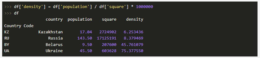
Теперь представим, что новый столбец нас чем-то не устраивает. Не беда — его можно без проблем удалить:

Ну а если вы очень ленивы, то достаточно написать del df[‘density’].
Для переименования столбцов воспользуемся методом rename:
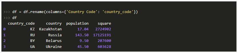
В вышеприведенном примере перед переименованием столбца Country Code следует сначала удостовериться, что с него сброшен индекс. В обратном случае никакого эффекта не будет.
Библиотека Pandas
Мы начинаем курс анализа и обработки данных. На двух предыдущих курсах мы, во-первых, получили общее представление о том, как устроено машинное обучение, и, во-вторых, приобрели достаточно продвинутые навыки в программировании на Питоне.
Курс анализа данных — это первый курс, в рамках которого мы переходим непосредственно к работе над построением моделей.
Для того чтобы лучше понимать содержание этого курса давайте вначале рассмотрим этапы построения модели.
Задача машинного обучения
Ниже представлена общая последовательность работы над задачей машинного обучения.

Описанный процесс принято называть пайплайном, то есть порядком действий (от англ. pipeline, трубопровод, конвейер), которые необходимо выполнять для построения модели. Подробнее рассмотрим некоторые из этих этапов.
Этап 1. Постановка задачи и определение метрики
Первый этап может показаться тривиальным, однако во многих случах, особенно в задачах классификации, выбор правильной метрики является ключевым для построения качественной модели. Про важность классификационной метрики мы начали говорить в рамках вводного курса и продолжим этот разговор в дальнейшем на гораздо более детальном уровне.
Этап 2. Получение данных
Важный этап. Хотя на этом курсе мы будем использовать уже готовые (зачастую учебные) датасеты, стоит помнить, что получение данных (data gathering) не происходит само собой и во многом от того как и какие данные собраны будет зависеть конечный результат (на который не смогут повлиять ни качественный EDA, ни сложный алгоритм машинного обучения).
Этап 3. Исследовательский анализ данных
В рамках EDA нам нужно решить три основных задачи: описать данные, найти отличия и выявить взаимосвязи. Описание данных позволяет понять, о каких данных идет речь, а также выявить недостатки в данных (с которыми мы справляемся на этапе обработки). Отличия и взаимосвязи в данных — основа для построения модели, это то, за что модель «цепляется», чтобы выдать верный числовой результат, правильную классификацию или кластер.
Для решения этих задач наилучшим образом подходят средства визуализации и описательная статистика. Этим мы займемся во втором разделе.
Отдельно хочется сказать про baseline models, простые модели, которые мы строим в самом начале работы. Они позволяют понять какой результат мы можем получить, не вкладывая дополнительных усилий в работу с данными, а затем отталкиваться от этого результата для обработки данных и построения более сложных моделей.
Базовые модели мы начнем строить на курсе по оптимизации.
Этап 4. Обработка данных
Как уже было сказано, на этапе EDA зачастую становится очевидно, что в данных есть недостатки, которые сильно повляют на качество модели или в целом не позволят ее обучить.
Очистка данных: ошибки и пропуски
Во-первых, в данных могут встречаться ошибки: дубликаты, неверные значения или неподходящий формат данных. Кроме того, данные могут содержать пропуски, и с ними также нужно что-то делать. Этим вопросам посвящен третий раздел курса.
Преобразование данных
Во-вторых, зачастую количественные данные нужно привести к одному масштабу и/или нормальному распределению. Кроме того, числовые признаки могут содержать сильно отличающиеся от остальных данных значения или выбросы, которые также повляют на конечный результат. Категориальные данные необходимо закодировать с помощью чисел. Если категориальные данные выражены строками, это может воспрепятствовать обучению алгоритма.
Преобразование количественных и категориальных данных рассматривается в четвертом разделе.
Конструирование и отбор признаков, понижение размерности
Еще одним важным этапом является конструирование признаков, а также отбор признаков и понижение размерности. В рамках этого курса мы затронем лишь базовые способы конструирования признаков. Более сложные вопросы отбора признаков и понижения размерности мы отложим на потом.
Этап 5. Моделирование и оценка результата
Когда данные готовы, их можно загружать в модель, обучать эту модель и оценивать результат.
Здесь важно сказать, что это итеративный (iterative) или циклический процесс. Многие из описанных выше шагов могут повторяться. В частности, построение модели может привести к необходимости дополнительной обработки данных. Кроме того, разные алгоритмы требуют разной подготовки данных (например, линейные модели требуют масштабирования данных, а для деревьев решений этого не нужно).
При этом прежде чем приступить к анализу и обработке данных важно освоить библиотеку Pandas. Именно этим мы и займемся в начале курса.
Про библиотеку Pandas
Библиотека Pandas — это ключевой инструмент для анализа данных на Питоне. Она позволяет работать с данными, представленными в табличной форме, а также временными рядами. Как вы уже видели, Pandas легко интегрируется с matplotlib, seaborn, sklearn и другими библиотеками.
Кроме того, структурно изучение Pandas можно разделить на два больших раздела: преобразование данных и статистический анализ. В этом разделе (текущее и следующее занятие) мы начнем знакомиться с первой частью, а в следующем (занятия три и четыре) перейдем ко второй.
Объекты DataFrame и Series
В Pandas есть два основных объекта: DataFrame и Series. Слегка упрощая, можно сказать, что DataFrame — это таблица (и соответственно двумерный массив), а Series — столбец этой таблицы (а значит одномерный массив).

Индекс (index), столбцы (columns) и значения (values) датафрейма мы разберем чуть позднее, а сейчас давайте посмотрим на способы создания датафрейма.
Создание датафрейма
Способ 1. Создание датафрейма из файла
Датафрейм можно создать, импортировав файлы различных форматов. Мы уже делали так с файлами в формате .csv с помощью функции pd.read_csv(). Аналогичным образом можно импортировать файлы и в других форматах, например MS Excel или html. Рассмотрим несколько примеров.
Файл .csv в zip-архиве. Если в zip-архиве содержится только один файл, его можно напрямую подгрузить в Pandas. Вначале скачаем необходимые данные.
После скачивания не забудьте подгрузить данные в сессионное хранилище Google Colab.