Решаем задачу численного прогнозирования с помощью линейной регрессии на Python

Задача регрессии возникает, когда требуется предсказать цену, температура, пульс, время, давление или другое численный показатель. Это пример контролируемого (supervised) машинного обучения, когда на основе истории предыдущих данных мы получаем предсказание. В этой статье обсудим, как можно спрогнозировать будущее, решая задачу линейной регрессии на Python.
Постановка задачи и исходный датасет
Продолжим работу с датасетом нью-йоркских апартаментов (отелей), доступных для проживания на некоторое время. Для дальнейшего анализа возьмем район Бруклин:
import pandas as pd data = pd.read_csv(‘../AB_NYC_2019.csv’) data = data[data[‘neighbourhood_group’] == ‘Brooklyn’]
На этом наборе данных будем прогнозировать цены, по которым можно арендовать отдельные аппартаменты.
Линейная регрессия с одной независимой переменной
Графически линейная регрессия с одной независимой выглядит как прямая. Она решает задачу регрессии нахождением прямой, которая наилучшим образом соответствует точкам наблюдений. Следующий рисунок иллюстрирует вышесказанное:
Линейная регрессия (красная линия) наиболее полно соответствует точкам
Модель линейной регрессии может быть задана следующим образом:
Следовательно, для решения задачи регрессии требуется найти коэффициенты $a$ (коэффициент наклона) и $b$ (точка пересечения линии с осью ординат). Не вдаваясь в подробности, их можно выразить так:
Найдем коэффициенты в Python, написав следующие функции:
def calculate_slope(x, y):
return sum(mx * my) / sum(mx**2)
def get_params(x, y):
a = calculate_slope(x, y)
b = y.mean() — a * x.mean()
Стоит заметить, функция calculate_slope сначала находит произведение двух массивов, только потом суммирует результат этого произведения.
В нашем случае выберем в качестве независимой переменной $x$ — количество отзывов number_of_reviews, a зависимой переменной $y$, которую требуется предсказать, будет цена price. Кроме того, чтобы избежать излишней волатильности цены, мы ее прологарифмируем, как это объяснялось в прошлый раз. Посмотрим на полученные коэффициенты:
>>> import numpy as np
import numpy as np
d = data[data.price > 0]
y = np.log(d.price) a, b = get_params(x, y)
В итоге получили:
>>> a -0.04213862786693919 >>> b 125.40308200933784
Мы отфильтровали нулевые значения цены, так как логарифма от нуля не существует. Таким образом, линейная регрессия будет задаваться как:
Построим график в Python-библиотеке matplotlib, на котором будет видна полученная линейная регрессия и истинные значения цены. О том, как строить графики, мы рассказывали тут. Для этого воспользуемся функциями scatter и plot:
import matplotlib.pyplot as plt
plt.ylabel(‘Цена в логарифмическом масштабе’)
plt.plot(x, lin_reg, color=’red’)
В результате получили график:
Линейная регрессия (красная линия)
Как можно заметить, линейная регрессия с одной независимой переменной показывает неудачные результаты, так как является практически параллельной оси абсцисс. Поэтому предсказание будет одним и тем же, примерно равным 4.6. При переводе обратно в нормальный масштаб равняется \$100.
Линейная регрессия в библиотеках statsmodel и seaborn
Чтобы получить линейную регрессию, Data Scientist, который работает с Python, может воспользоваться готовыми библиотеками, а не писать собственное решение. Например, отлично подойдет библиотека Statsmodel, о которой мы уже говорили здесь. Она позволит получить линейную регрессию очень быстро:
import statsmodels.formula.api as smf
res = model.fit() res.summary()
Метод summary выдает резюме после вычислений линейной регрессии по методу наименьших квадратов. Но нас интересуют коэффициенты $a$ и $b$, которые в данном случае равны:
Коэффициенты линейной регрессии
Как видим, intercept — это $b$, number_of reviews, — это $a$, что соответствуют прошлым вычислениям.
Помимо Statsmodel, можно воспользоваться библиотекой Seaborn, которая также часто применяется в задачах Machine Learning и других методах Data Science. Она имеет функцию regplot, которая сразу построит соответствующую прямую:
import seaborn as sns
Линейная регрессия с несколькими переменными в Scikit-learn
В действительности ML-модели редко обучаются только на одном признаке, что подтверждают построенные графики. Поэтому уравнение для линейной регрессии можно обобщить до $n$ переменных (признаков):
\[
y = ax_1 + ax_2 \dots + \dots + ax_n
\]
где задача сводится к нахождению коэффициентов. Не вдаваясь в подробности их нахождения, отметим, что Python-библиотека Scikit-learn предоставляет для этого уже готовый интерфейс.
Рассмотрим пример в Python. Выберем в качестве независимых переменных признаки: number_of_reviews, reviews_per_month, calculated_host_listings_count. Атрибут reviews_per_month имеет Nan-значения, поэтому в дальнейшем заполним их нулями. К тому же, мы отфильтровали те данные, которые имеют нулевую цену:
d = data[data.price > 0]
x = d.loc[:, (‘reviews_per_month’, ‘calculated_host_listings_count’, ‘number_of_reviews’)]
Здесь используется метод loc, который, согласно документации, быстрее и производительнее явного вызова столбцов [1]. Нам также требуется разбить полученные данные на тренировочную и тестовую выборки, чтобы на одних данных обучить модель, а на других — проверить ее корректность. В Scikit-learn имеется функция train_test_split, возвращающая две пары массивов — тренировочного и тестового:
from sklearn.model_selection import train_test_split
x_train, x_test, y_train, y_test = train_test_split(x, y, test_size=0.2)
Данная функция принимает в качестве аргумента также test_size, который определяет долю, отведенную на тестовую выборку.
Теперь к самому главному — обучению модели линейной регрессии. В Scikit-learn есть класс LinearRegression, который выполнит за нас работу в Python:
from sklearn.linear_model import LinearRegression
model = LinearRegression().fit(x_train, y_train)
В метод fit мы посылаем те данные, на которых ML-модель обучается. Попробуем получить предсказания на основе тестовой выборки:
А как узнать, что такая модель лучшая из всех доступных? Нужно воспользоваться метриками качества.
Метрики качества для оценки работоспособности модели
Чтобы оценить работоспособность модели, применяют специальные метрики. Для задачи регрессии применяют среднеквадратическую (MSE) и абсолютную ошибки (MAE). Среднеквадратическая ошибка находится как:
MSE =sum(y-y_
Абсолютная опускает возведение в квадрат:
MAE = sum|y-y_
Перед оценкой стоит экспонировать тестовые и пересказанные значения, так как использовать MAE и MSE для логарифмов будет нецелесообразно, поскольку трудно будет оценить полученные результаты. Поэтому проделаем следующее:
В модуле metrics имеется соответственно mean_squared_error, mean_absolute_error:
from sklearn.metrics import mean_squared_error
from sklearn.metrics import mean_absolute_error
mse = mean_squared_error(y_test, y_pred)
mae = mean_absolute_error(y_test, y_pred)
print(‘mse: %.3f, mae: %.3f’ % (mse, mae))
В результате мы получили соответствующие результаты:
Абсолютная ошибка составляет $63, a если взять корень от среднеквадратической ошибки, то получится \$182. В целом, это большие значения, особенно с перерасчетом в рубли. Что можно сделать, чтобы улучшить модель? Здесь можно применить следующее:
Использовать другие модели MachineLearning, в Scikit-learn их огромное количество [2]; отфильтровать данные, например, взять только те места, в которых можно остаться только на 1–2 ночи или, наоборот, на 1 месяц; добавить дополнительные признаки.
Смотрите в видеообзоре, как можно обработать данные, а также как добавить геокоординаты в качестве дополнительных признаков.
Как эффективно решать задачи линейной регрессии, а также работать с другими методами Machine Learning с помощью Python, вы узнаете на практических курсах для специалистов Big Data в нашем лицензированном учебном центре обучения и повышения квалификации ИТ-специалистов в Москве.
Линейная регрессия с помощью Scikit-Learn в Python
Существует два типа алгоритмов машинного обучения с учителем: регрессия и классификация. Первый прогнозирует непрерывные выходы значений, а второй – дискретные. Например, прогнозирование стоимости дома в долларах является проблемой регрессии, тогда как прогнозирование злокачественной или доброкачественной опухоли является проблемой классификации.
В этой статье мы кратко изучим, что такое линейная регрессия и как ее можно реализовать с помощью библиотеки Python Scikit-Learn, которая является одной из самых популярных библиотек машинного обучения для Python.
Теория линейной регрессии
Термин «линейность» в алгебре относится к линейной зависимости между двумя или более переменными. Если мы нарисуем это соотношение в двухмерном пространстве (в данном случае между двумя переменными), мы получим прямую линию.
Давайте рассмотрим скрипт, в котором мы хотим определить линейную зависимость между количеством часов, которые студент учится, и процентом оценок, которые студент набирает на экзамене. Мы хотим выяснить, сколько часов ученик готовится к тесту, насколько высокий балл он может набрать? Если мы нанесем независимую переменную (часы) на ось x, а зависимую переменную (процент) на ось y, линейная регрессия даст нам прямую линию, которая наилучшим образом соответствует точкам данных, как показано на рисунке ниже.

Мы знаем, что уравнение прямой в основном:
Где, b – точка пересечения, а m – наклон линии. Таким образом, алгоритм линейной регрессии дает нам наиболее оптимальное значение для точки пересечения и наклона (в двух измерениях). Переменные y и x остаются неизменными, поскольку они являются функциями данных и не могут быть изменены. Значения, которые мы можем контролировать, – это точка пересечения и наклон. В зависимости от значений точки пересечения и наклона может быть несколько прямых линий. По сути, алгоритм линейной регрессии помещает несколько строк в точки данных и возвращает строку, которая дает наименьшую ошибку.
Эту же концепцию можно распространить на случаи, когда существует более двух переменных. Это называется множественной линейной регрессией. Например, рассмотрим скрипт, в котором вы должны спрогнозировать цену дома на основе его площади, количества спален, среднего дохода людей в этом районе, возраста дома и т.д. В этом случае зависимая переменная зависит от нескольких независимых переменных. Модель регрессии, включающая несколько переменных, может быть представлена как:
Это уравнение гиперплоскости. Помните, что модель линейной регрессии в двух измерениях – это прямая линия, в трех измерениях – это плоскость, а в более чем трех измерениях – гиперплоскость.
Линейная регрессия
В этом разделе мы увидим, как библиотеку Scikit-Learn в Python для машинного обучения можно использовать для реализации функций регрессии. Мы начнем с простой линейной регрессии с участием двух переменных, а затем перейдем к линейной регрессии с участием нескольких переменных.
Простая линейная регрессия
В этой задаче регрессии мы спрогнозируем процент оценок, которые, как ожидается, получит студент, на основе количества часов, которые он изучил. Это простая задача линейной регрессии, поскольку она включает всего две переменные.
Импорт библиотек
Чтобы импортировать необходимые библиотеки для этой задачи, выполните следующие операторы импорта:
Примечание. Как вы могли заметить из приведенных выше операторов импорта, этот код был выполнен с использованием Jupyter iPython Notebook.
Набор данных
Примечание. Этот пример был выполнен на компьютере под управлением Windows, и набор данных хранился в папке «D:\datasets». Вы можете скачать файл в другом месте, если соответствующим образом измените путь к набору данных.
Следующая команда импортирует набор данных CSV с помощью Pandas:
Теперь давайте немного исследуем наш набор данных. Для этого выполните следующий скрипт:
После этого вы должны увидеть следующее:
Это означает, что в нашем наборе данных 25 строк и 2 столбца. Давайте посмотрим, как на самом деле выглядит наш набор данных. Для этого используйте метод head():
Вышеупомянутый метод извлекает первые 5 записей из нашего набора данных, которые будут выглядеть следующим образом:
| Часы | Очки | |
|---|---|---|
| 0 | 2,5 | 21 год |
| 1 | 5.1 | 47 |
| 2 | 3,2 | 27 |
| 3 | 8,5 | 75 |
| 4 | 3.5 | 30 |
Чтобы увидеть статистические детали набора данных, мы можем использовать description():
| Часы | Очки | |
|---|---|---|
| count | 25,000000 | 25,000000 |
| mean | 5,012000 | 51,480000 |
| std | 2,525094 | 25,286887 |
| min | 1 100 000 | 17,000000 |
| 25% | 2,700000 | 30,000000 |
| 50% | 4,800000 | 47,000000 |
| 75% | 7,400000 | 75,000000 |
| max | 9.200000 | 95,000000 |
И, наконец, давайте нарисуем наши точки данных на двухмерном графике, чтобы взглянуть на наш набор данных и посмотреть, сможем ли мы вручную найти какую-либо связь между данными. Мы можем создать сюжет с помощью следующего скрипта:
В приведенном выше скрипте мы используем функцию plot() dataframe pandas и передаем ей имена столбцов для координаты x и координаты y, которые являются «часами» и «счетами» соответственно.
В результате сюжет будет выглядеть так:

Из приведенного выше графика мы можем ясно видеть, что существует положительная линейная зависимость между количеством изученных часов и процентом набранных баллов.
Подготовка данных
Теперь у нас есть представление о статистических деталях наших данных. Следующим шагом является разделение данных на «атрибуты» и «метки». Атрибуты – это независимые переменные, а метки – это зависимые переменные, значения которых должны быть предсказаны. В нашем наборе данных всего два столбца. Мы хотим предсказать процентную оценку в зависимости от изученных часов. Поэтому наш набор атрибутов будет состоять из столбца «Часы», а меткой будет столбец «Оценка». Чтобы извлечь атрибуты и метки, выполните следующий сценарий:
Атрибуты хранятся в переменной X. Мы указали «-1» в качестве диапазона для столбцов, так как мы хотели, чтобы наш атрибут содержал все столбцы, кроме последнего, которым является «Результаты». Точно так же переменная y содержит метки. Мы указали 1 для столбца метки, так как индекс столбца «Результаты» равен 1. Помните, что индексы столбца начинаются с 0, причем 1 является вторым столбцом. В следующем разделе мы увидим лучший способ указать столбцы для атрибутов и меток.
Теперь, когда у нас есть атрибуты и метки, следующим шагом будет разделение этих данных на обучающий и тестовый наборы. Мы сделаем это с помощью встроенного в Scikit-Learn метода train_test_split():
Приведенный выше скрипт разделяет 80% данных на обучающий набор, а 20% данных – на набор тестов. Переменная test_size -–это то место, где мы фактически указываем пропорцию набора тестов.
Обучение алгоритму
Мы разделили наши данные на наборы для обучения и тестирования, и теперь, наконец, пришло время обучить наш алгоритм. Выполните следующую команду:
С Scikit-Learn чрезвычайно просто реализовать модели линейной регрессии, поскольку все, что вам действительно нужно сделать, это импортировать класс LinearRegression, создать его экземпляр и вызвать метод fit() вместе с нашими обучающими данными. Это примерно так же просто, как и при использовании библиотеки машинного обучения.
В разделе теории мы сказали, что модель линейной регрессии в основном находит наилучшее значение для точки пересечения и наклона, в результате чего получается линия, которая наилучшим образом соответствует данным. Чтобы увидеть значение точки пересечения и наклона, вычисленное алгоритмом линейной регрессии для нашего набора данных, выполните следующий код.
Чтобы получить перехват:
Полученное значение должно быть примерно 2,01816004143.
Для получения наклона (коэффициента x):
Результат должен быть примерно 9.91065648.
Это означает, что на каждую единицу изменения в изученных часах изменение оценки составляет около 9,91%. Или, проще говоря, если студент учится на один час больше, чем готовился к экзамену ранее, он может рассчитывать на повышение на 9,91% баллов, полученных студентом ранее.
Прогнозы
Теперь, когда мы обучили наш алгоритм, пришло время сделать некоторые прогнозы. Для этого мы воспользуемся нашими тестовыми данными и посмотрим, насколько точно наш алгоритм предсказывает процентную оценку. Чтобы сделать прогнозы на тестовых данных, выполните следующий скрипт:
Y_pred – это массив numpy, который содержит все предсказанные значения для входных значений в серии X_test.
Чтобы сравнить фактические выходные значения для X_test с прогнозируемыми значениями, выполните следующий скрипт:
Результат выглядит так:
| Действительный | Прогнозируемый | |
|---|---|---|
| 0 | 20 | 16,884145 |
| 1 | 27 | 33,732261 |
| 2 | 69 | 75.357018 |
| 3 | 30 | 26.794801 |
| 4 | 62 | 60,491033 |
Хотя наша модель не очень точна, прогнозируемые проценты близки к фактическим.
Значения в вышеприведенных столбцах могут отличаться в вашем случае, потому что функция train_test_split случайным образом разбивает данные на обучающие и тестовые наборы, и ваши разбиения, вероятно, будут отличаться от показанного в этой статье.
Оценка алгоритма
- Средняя абсолютная ошибка (MAE) – это среднее абсолютное значение ошибок. Он рассчитывается как:
- Среднеквадратичная ошибка (MSE) – это среднее значение квадратов ошибок, которое рассчитывается как:
- Среднеквадратичная ошибка (RMSE) – это квадратный корень из среднего квадрата ошибок:

К счастью, нам не нужно выполнять эти вычисления вручную. Библиотека Scikit-Learn поставляется со встроенными функциями, которые можно использовать, чтобы узнать эти значения для нас.
Давайте найдем значения этих показателей, используя наши тестовые данные. Выполните следующий код:
Результат будет выглядеть примерно так (но, вероятно, немного иначе):
Вы можете видеть, что значение среднеквадратичной ошибки составляет 4,64, что составляет менее 10% от среднего значения процентов всех студентов, т.е. 51,48. Это означает, что наш алгоритм проделал достойную работу.
Множественная линейная регрессия
В предыдущем разделе мы выполнили линейную регрессию с участием двух переменных. Почти все проблемы реального мира, с которыми вы столкнетесь, будут иметь более двух переменных. Линейная регрессия с участием нескольких переменных называется «множественной линейной регрессией». Шаги по выполнению множественной линейной регрессии почти аналогичны шагам простой линейной регрессии. Разница заключается в оценке. Вы можете использовать его, чтобы узнать, какой фактор имеет наибольшее влияние на прогнозируемый результат и как разные переменные связаны друг с другом.
В этом разделе мы будем использовать множественную линейную регрессию для прогнозирования потребления газа (в миллионах галлонов) в 48 штатах США на основе налогов на газ (в центах), дохода на душу населения (в долларах), дорог с твердым покрытием (в милях) и доли население, имеющее водительские права.
Первые два столбца в приведенном выше наборе данных не предоставляют никакой полезной информации, поэтому они были удалены из файла набора данных. Теперь давайте разработаем регрессионную модель для этой задачи.
Импорт библиотек
Следующий скрипт импортирует необходимые библиотеки:
Набор данных
Следующая команда импортирует набор данных из файла:
Как и в прошлый раз, давайте посмотрим, как на самом деле выглядит наш набор данных. Выполните команду head():
Первые несколько строк нашего набора данных выглядят так:
| Petrol_tax | Средний заработок | Асфальтированные, шоссе | Population_Driver_license (%) | Petrol_Consumption | |
|---|---|---|---|---|---|
| 0 | 9.0 | 3571 | 1976 г. | 0,525 | 541 |
| 1 | 9.0 | 4092 | 1250 | 0,572 | 524 |
| 2 | 9.0 | 3865 | 1586 | 0,580 | 561 |
| 3 | 7,5 | 4870 | 2351 | 0,529 | 414 |
| 4 | 8.0 | 4399 | 431 | 0,544 | 410 |
Чтобы увидеть статистические детали набора данных, мы снова воспользуемся командой describe():
| Petrol_tax | Средний заработок | Асфальтированные, шоссе | Population_Driver_license (%) | Petrol_Consumption | |
|---|---|---|---|---|---|
| count | 48,000000 | 48,000000 | 48,000000 | 48,000000 | 48,000000 |
| mean | 7,668333 | 4241.833333 | 5565.416667 | 0,570333 | 576.770833 |
| std | 0,950770 | 573,623768 | 3491.507166 | 0,055470 | 111,885816 |
| min | 5,000000 | 3063.000000 | 431,000000 | 0,451000 | 344,000000 |
| 25% | 7,000000 | 3739.000000 | 3110.250000 | 0,529750 | 509 500 000 |
| 50% | 7,500000 | 4298.000000 | 4735.500000 | 0,564500 | 568 500 000 |
| 75% | 8,125 000 | 4578.750000 | 7156.000000 | 0,595250 | 632,750000 |
| max | 10,00000 | 5342.000000 | 17782,000000 | 0,724000 | 986,000000 |
Подготовка данных
Следующим шагом является разделение данных на атрибуты и метки, как мы делали ранее. Однако, в отличие от прошлого раза, на этот раз мы собираемся использовать имена столбцов для создания набора атрибутов и метки. Выполните следующий скрипт:
Выполните следующий код, чтобы разделить наши данные на обучающий и тестовый наборы:
Обучение алгоритму
И, наконец, для обучения алгоритма мы выполняем тот же код, что и раньше, используя метод fit() класса LinearRegression:
Как было сказано ранее, в случае многомерной линейной регрессии регрессионная модель должна найти наиболее оптимальные коэффициенты для всех атрибутов. Чтобы увидеть, какие коэффициенты выбрала наша регрессионная модель, выполните следующий скрипт:
Результат должен выглядеть примерно так:
| Коэффициент | |
|---|---|
| Petrol_tax | -24.196784 |
| Average_income | -0,81680 |
| Paved_Highways | -0,000522 |
| Population_Driver_license (%) | 1324.675464 |
Это означает, что увеличение “petrol_tax” на единицу приводит к снижению потребления газа на 24,19 миллиона галлонов. Аналогичным образом, увеличение доли населения, имеющего водительские права, приводит к увеличению потребления газа на 1,324 миллиарда галлонов. Мы видим, что «Average_income» и «Paved_Highways» очень мало влияют на потребление газа.
Прогнозы
Чтобы сделать прогнозы на тестовых данных, выполните следующий скрипт:
Чтобы сравнить фактические выходные значения для X_test с прогнозируемыми значениями, выполните следующий скрипт:
Результат выглядит так:
| Действительный | Прогнозируемый | |
|---|---|---|
| 36 | 640 | 643.176639 |
| 22 | 464 | 411.950913 |
| 20 | 649 | 683,712762 |
| 38 | 648 | 728.049522 |
| 18 | 865 | 755.473801 |
| 1 | 524 | 559.135132 |
| 44 год | 782 | 671.916474 |
| 21 год | 540 | 550,633557 |
| 16 | 603 | 594,425464 |
| 45 | 510 | 525.038883 |
Оценка алгоритма
Последний шаг – оценить производительность алгоритма. Мы сделаем это, найдя значения для MAE, MSE и RMSE. Выполните следующий скрипт:
Результат будет выглядеть примерно так:
Вы можете видеть, что значение среднеквадратичной ошибки составляет 60,07, что немного больше 10% от среднего значения потребления газа во всех штатах. Это означает, что наш алгоритм не был очень точным, но все же может делать достаточно хорошие прогнозы.
- Требуется больше данных: данных за один год – это не так уж и много, тогда как накопление данных за несколько лет могло бы помочь нам немного повысить точность.
- Ошибочные предположения: мы предположили, что эти данные имеют линейную зависимость, но это может быть не так. Визуализация данных может помочь вам определить это.
- Плохие функции: используемые нами функции могли не иметь достаточно высокой корреляции со значениями, которые мы пытались предсказать.
Заключение
В этой статье мы изучили один из самых фундаментальных алгоритмов машинного обучения, то есть линейную регрессию. Мы реализовали как простую линейную регрессию, так и множественную линейную регрессию с помощью библиотеки машинного обучения Scikit-Learn.
Линейная регрессия. Разбор математики и реализации на python
Тема линейной регресии рассмотрена множество раз в различных источниках, но, как говорится, «нет такой избитой темы, которую нельзя ударить еще раз». В данной статье рассмотрим указанную тему, используя как математические выкладки, так и код python, пытаясь соблюсти баланс на грани простоты и должном уровне для понимания математических основ.
Линейная регрессия представляется из себя регриссионную модель зависимости одной (объясняемой, зависимой) переменной от другой или нескольких других переменных (фактров, регрессоров, независимых переменных) с линейной функцией зависимости. Рассмотрим модель линейной регрессии, при которой зависимая переменная зависит лишь от одного фактора, тогда функция, описывающуя зависимость y от x будет иметь следующий вид:
и задача сводится к нахождению весовых коэффициентов w0 и w1, таких что такая прямая максимально «хорошо» будет описывать исходные данные. Для этого зададим функцию ошибки, минимизация которой обеспечит подбор весов w0 и w1, используя метод наименьших квадратов:
или подставив уравнение модели
Минимизируем функцию ошибки MSE найдя частные производные по w0 и w1
И приравняв их к нулю получим систему уравнений, решение которой обеспечит минимизацию функции потерь MSE.
Раскроем сумму и с учетом того, что -2/n не может равняться нулю, приравняем к нулю вторые множители
Выразим w0 из первого уравнения
Подставив во второе уравнение решим относительно w1
И выразив w1 последнего уравнения получим
Задача решена, однако представленный способ слабо распространим на большое количество фичей, уже при появлении второго признака вывод становится достаточно громоздким, не говоря уже о большем количестве признаков.
Справиться с этой задачей нам поможет матричный способ представления функции потерь и ее минимизация путем дифференцирования и нахождения экстремума в матричном виде.
Предположим, что дана следующая таблица с данными
17. Linear regression
The goal in this chapter is to introduce linear regression. Stripped to its bare essentials, linear regression models are basically a slightly fancier version of the Pearson correlation , though as we’ll see, regression models are much more powerful tools.
Since the basic ideas in regression are closely tied to correlation, we’ll return to the parenthood.csv file that we were using to illustrate how correlations work. Recall that, in this data set, we were trying to find out why Dan is so very grumpy all the time, and our working hypothesis was that I’m not getting enough sleep.
| dan_sleep | baby_sleep | dan_grump | day | |
|---|---|---|---|---|
| 0 | 7.59 | 10.18 | 56 | 1 |
| 1 | 7.91 | 11.66 | 60 | 2 |
| 2 | 5.14 | 7.92 | 82 | 3 |
| 3 | 7.71 | 9.61 | 55 | 4 |
| 4 | 6.68 | 9.75 | 67 | 5 |
We drew some scatterplots to help us examine the relationship between the amount of sleep I get, and my grumpiness the following day.
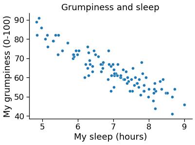
Fig. 17.1 Scatterplot showing grumpiness as a function of hours slept. 
The actual scatterplot that we draw is the one shown in Fig. 17.1 , and as we saw previously this corresponds to a correlation of \(r=-.90\) , but what we find ourselves secretly imagining is something that looks closer to the left panel in Fig. 17.2 . That is, we mentally draw a straight line through the middle of the data. In statistics, this line that we’re drawing is called a regression line. Notice that – since we’re not idiots – the regression line goes through the middle of the data. We don’t find ourselves imagining anything like the rather silly plot shown in the right panel in Fig. 17.2 .
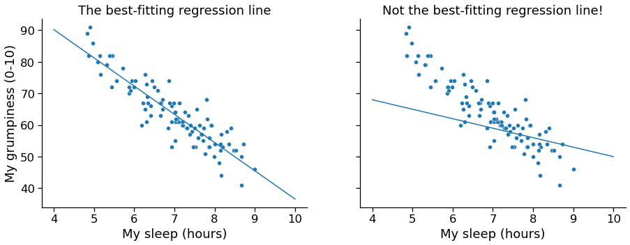
Fig. 17.2 The panel to the left shows the sleep-grumpiness scatterplot from Fig. 17.1 with the best fitting regression line drawn over the top. Not surprisingly, the line goes through the middle of the data. In contrast, the panel to the right shows the same data, but with a very poor choice of regression line drawn over the top. 
This is not highly surprising: the line that I’ve drawn in panel to the right doesn’t “fit” the data very well, so it doesn’t make a lot of sense to propose it as a way of summarising the data, right? This is a very simple observation to make, but it turns out to be very powerful when we start trying to wrap just a little bit of maths around it. To do so, let’s start with a refresher of some high school maths. The formula for a straight line is usually written like this:
Or, at least, that’s what it was when I went to high school all those years ago. The two variables are \(x\) and \(y\) , and we have two coefficients, \(m\) and \(c\) . The coefficient \(m\) represents the slope of the line, and the coefficient \(c\) represents the \(y\) -intercept of the line. Digging further back into our decaying memories of high school (sorry, for some of us high school was a long time ago), we remember that the intercept is interpreted as “the value of \(y\) that you get when \(x=0\) ”. Similarly, a slope of \(m\) means that if you increase the \(x\) -value by 1 unit, then the \(y\) -value goes up by \(m\) units; a negative slope means that the \(y\) -value would go down rather than up. Ah yes, it’s all coming back to me now.
Now that we’ve remembered that, it should come as no surprise to discover that we use the exact same formula to describe a regression line. If \(Y\) is the outcome variable (the DV) and \(X\) is the predictor variable (the IV), then the formula that describes our regression is written like this:
Hm. Looks like the same formula, but there’s some extra frilly bits in this version. Let’s make sure we understand them. Firstly, notice that I’ve written \(X_i\) and \(Y_i\) rather than just plain old \(X\) and \(Y\) . This is because we want to remember that we’re dealing with actual data. In this equation, \(X_i\) is the value of predictor variable for the \(i\) th observation (i.e., the number of hours of sleep that I got on day \(i\) of my little study), and \(Y_i\) is the corresponding value of the outcome variable (i.e., my grumpiness on that day). And although I haven’t said so explicitly in the equation, what we’re assuming is that this formula works for all observations in the data set (i.e., for all \(i\) ). Secondly, notice that I wrote \(\hat
Excellent, excellent. Next, I can’t help but notice that – regardless of whether we’re talking about the good regression line or the bad one – the data don’t fall perfectly on the line. Or, to say it another way, the data \(Y_i\) are not identical to the predictions of the regression model \(\hat
which in turn means that we can write down the complete linear regression model as:
17.1. Estimating a linear regression model
Okay, now let’s redraw our pictures, but this time I’ll add some lines to show the size of the residual for all observations. When the regression line is good, our residuals (the lengths of the solid black lines) all look pretty small, as shown in the left panel of Fig. 17.3 , but when the regression line is a bad one, the residuals are a lot larger, as you can see from looking at the right panel of Fig. 17.3 . Hm. Maybe what we “want” in a regression model is small residuals. Yes, that does seem to make sense. In fact, I think I’ll go so far as to say that the “best fitting” regression line is the one that has the smallest residuals. Or, better yet, since statisticians seem to like to take squares of everything why not say that …
The estimated regression coefficients, \(\hat_0\) and \(\hat_1\) are those that minimise the sum of the squared residuals, which we could either write as \(\sum_i (Y_i — \hat
Yes, yes that sounds even better. And since I’ve indented it like that, it probably means that this is the right answer. And since this is the right answer, it’s probably worth making a note of the fact that our regression coefficients are estimates (we’re trying to guess the parameters that describe a population!), which is why I’ve added the little hats, so that we get \(\hat_0\) and \(\hat_1\) rather than \(b_0\) and \(b_1\) . Finally, I should also note that – since there’s actually more than one way to estimate a regression model – the more technical name for this estimation process is ordinary least squares (OLS) regression.
At this point, we now have a concrete definition for what counts as our “best” choice of regression coefficients, \(\hat_0\) and \(\hat_1\) . The natural question to ask next is, if our optimal regression coefficients are those that minimise the sum squared residuals, how do we find these wonderful numbers? The actual answer to this question is complicated, and it doesn’t help you understand the logic of regression.2 As a result, this time I’m going to let you off the hook. Instead of showing you how to do it the long and tedious way first, and then “revealing” the wonderful shortcut that Python provides you with, let’s cut straight to the chase… and use Python to do all the heavy lifting.
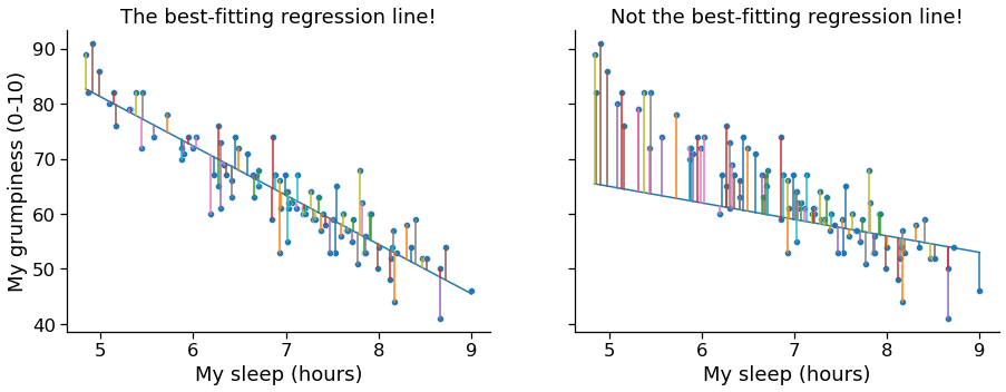
Fig. 17.3 A depiction of the residuals associated with the best fitting regression line (left panel), and the residuals associated with a poor regression line (right panel). The residuals are much smaller for the good regression line. Again, this is no surprise given that the good line is the one that goes right through the middle of the data. 
17.2. Linear Regression with Python
As always, there are several different ways we could go about calculating a linear regression in Python, but we’ll stick with pingouin , which for my money is one of the simplest and easiest packages to use. The pingouin command for linear regression is, well, linear_regression , so that couldn’t be much more straightforward. After that, we just need to tell pinguoin which variable we want to use as a predictor variable (independent variable), and which one we want to use as the outcome variable (dependent variable). pingouin wants the predictor variable first, so, since we want to model my grumpiness as a function of my sleep, we write:
| names | coef | se | T | pval | r2 | adj_r2 | CI[2.5%] | CI[97.5%] | |
|---|---|---|---|---|---|---|---|---|---|
| 0 | Intercept | 125.96 | 3.02 | 41.76 | 0.0 | 0.82 | 0.81 | 119.97 | 131.94 |
| 1 | dan_sleep | -8.94 | 0.43 | -20.85 | 0.0 | 0.82 | 0.81 | -9.79 | -8.09 |
As is its way, pingouin gives us a nice simple table, with a lot of information. Most importantly for now, we can see that pingouin has caclulated the intercept \(\hat_0 = 125.96\) and the slope \(\hat_1 = -8.94\) . In other words, the best-fitting regression line that I plotted in Fig. 17.2 has this formula:
17.2.1. Warning. 
Remember, it’s critical that you put the variables in the right order. If you reverse the predictor and outcome variables, pinguoin will happily calculate a result for you, but it will not be the one you are looking for. If instead, we had written pg.linear_regression(df[‘dan_grump’], df[‘dan_sleep’]) , we would get the following:
| names | coef | se | T | pval | r2 | adj_r2 | CI[2.5%] | CI[97.5%] | |
|---|---|---|---|---|---|---|---|---|---|
| 0 | Intercept | 12.78 | 0.28 | 45.27 | 0.0 | 0.82 | 0.81 | 12.22 | 13.34 |
| 1 | dan_grump | -0.09 | 0.00 | -20.85 | 0.0 | 0.82 | 0.81 | -0.10 | -0.08 |
The output looks valid enough on the face of it, and it is even statistically significant. But in this model, we just predicted my son’s sleepiness as a function of my grumpiness, which is madness! Reversing the direction of causality would make a great scifi movie3, but it’s no good in statistics. So remember, predictor first, outcome second4
17.2.2. Interpreting the estimated model
The most important thing to be able to understand is how to interpret these coefficients. Let’s start with \(\hat_1\) , the slope. If we remember the definition of the slope, a regression coefficient of \(\hat_1 = -8.94\) means that if I increase \(X_i\) by 1, then I’m decreasing \(Y_i\) by 8.94. That is, each additional hour of sleep that I gain will improve my mood, reducing my grumpiness by 8.94 grumpiness points. What about the intercept? Well, since \(\hat_0\) corresponds to “the expected value of \(Y_i\) when \(X_i\) equals 0”, it’s pretty straightforward. It implies that if I get zero hours of sleep ( \(X_i =0\) ) then my grumpiness will go off the scale, to an insane value of ( \(Y_i = 125.96\) ). Best to be avoided, I think.
17.3. Multiple linear regression
The simple linear regression model that we’ve discussed up to this point assumes that there’s a single predictor variable that you’re interested in, in this case dan_sleep . In fact, up to this point, every statistical tool that we’ve talked about has assumed that your analysis uses one predictor variable and one outcome variable. However, in many (perhaps most) research projects you actually have multiple predictors that you want to examine. If so, it would be nice to be able to extend the linear regression framework to be able to include multiple predictors. Perhaps some kind of multiple regression model would be in order?
Multiple regression is conceptually very simple. All we do is add more terms to our regression equation. Let’s suppose that we’ve got two variables that we’re interested in; perhaps we want to use both dan_sleep and baby_sleep to predict the dan_grump variable. As before, we let \(Y_i\) refer to my grumpiness on the \(i\) -th day. But now we have two \(X\) variables: the first corresponding to the amount of sleep I got and the second corresponding to the amount of sleep my son got. So we’ll let \(X_
As before, \(\epsilon_i\) is the residual associated with the \(i\) -th observation, \(\epsilon_i =
17.4. Multiple Linear Regression in Python
Doing mulitiple linear regression in pingouin is just as easy as adding some more predictor variables, like this:
Still, there is one thing to watch out for. If you look carefully at the command above, you will notice that not only have we added a new predictor ( baby_sleep ), we have also added some extra brackets. While before our predictor variable was [‘dan_sleep’] , now we have [[‘dan_sleep’, ‘baby_sleep’]] . Why the extra set of [] ?
This is because we are using the brackets in two different ways. When we wrote [‘dan_sleep’] , the square brackets mean “select the column with the header ‘dan_sleep’”. But now we are giving pingouin a list of columns to select, and list objects are also defined by square brackets in Python. To keep things clear, another way to achieve the same result would be to define the list of predictor variables outside the call to pingouin :
You could do all the work outside of pinguoin , like this:
All three of these will give the same result, so it’s up to you choose what makes most sense to you. But now it’s time to take a look at the results:
| names | coef | se | T | pval | r2 | adj_r2 | CI[2.5%] | CI[97.5%] | |
|---|---|---|---|---|---|---|---|---|---|
| 0 | Intercept | 125.97 | 3.04 | 41.42 | 0.00 | 0.82 | 0.81 | 119.93 | 132.00 |
| 1 | dan_sleep | -8.95 | 0.55 | -16.17 | 0.00 | 0.82 | 0.81 | -10.05 | -7.85 |
| 2 | baby_sleep | 0.01 | 0.27 | 0.04 | 0.97 | 0.82 | 0.81 | -0.53 | 0.55 |
The coefficient associated with dan_sleep is quite large, suggesting that every hour of sleep I lose makes me a lot grumpier. However, the coefficient for baby_sleep is very small, suggesting that it doesn’t really matter how much sleep my son gets; not really. What matters as far as my grumpiness goes is how much sleep I get. To get a sense of what this multiple regression model looks like, Fig. 17.4 shows a 3D plot that plots all three variables, along with the regression model itself.
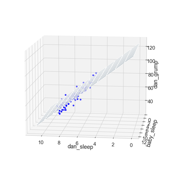
Fig. 17.4 A 3D visualisation of a multiple regression model. There are two predictors in the model, dan_sleep and baby_sleep ; the outcome variable is dan.grump . Together, these three variables form a 3D space: each observation (blue dots) is a point in this space. In much the same way that a simple linear regression model forms a line in 2D space, this multiple regression model forms a plane in 3D space. When we estimate the regression coefficients, what we’re trying to do is find a plane that is as close to all the blue dots as possible. 
17.4.1. Formula for the general case
The equation that I gave above shows you what a multiple regression model looks like when you include two predictors. Not surprisingly, then, if you want more than two predictors all you have to do is add more \(X\) terms and more \(b\) coefficients. In other words, if you have \(K\) predictor variables in the model then the regression equation looks like this:
17.5. Quantifying the fit of the regression model
So we now know how to estimate the coefficients of a linear regression model. The problem is, we don’t yet know if this regression model is any good. For example, the lm model claims that every hour of sleep will improve my mood by quite a lot, but it might just be rubbish. Remember, the regression model only produces a prediction \(\hat
17.5.1. The \(R^2\) value
Once again, let’s wrap a little bit of mathematics around this. Firstly, we’ve got the sum of the squared residuals:
which we would hope to be pretty small. Specifically, what we’d like is for it to be very small in comparison to the total variability in the outcome variable,
While we’re here, let’s calculate these values in Python. Firstly, in order to make my Python commands look a bit more similar to the mathematical equations, I’ll create variables X and Y :
First, lets just examine the output for the simple model that uses only a single predictor:
| names | coef | se | T | pval | r2 | adj_r2 | CI[2.5%] | CI[97.5%] | |
|---|---|---|---|---|---|---|---|---|---|
| 0 | Intercept | 125.96 | 3.02 | 41.76 | 0.0 | 0.82 | 0.81 | 119.97 | 131.94 |
| 1 | dan_sleep | -8.94 | 0.43 | -20.85 | 0.0 | 0.82 | 0.81 | -9.79 | -8.09 |
In this output, we can see that Python has calculated an intercept of 125.96 and a regression coefficient ( \(beta\) ) of -8.94. So for every hour of sleep I get, the model estimates that this will correspond to a decrease in grumpiness of about 9 on my incredibly scientific grumpiness scale. We can use this information to calculate \(\hat
Okay, now that we’ve got a variable which stores the regression model predictions for how grumpy I will be on any given day, let’s calculate our sum of squared residuals. We would do that using the following command:
Wonderful. A big number that doesn’t mean very much. Still, let’s forge boldly onwards anyway, and calculate the total sum of squares as well. That’s also pretty simple:
Hm. Well, it’s a much bigger number than the last one, so this does suggest that our regression model was making good predictions. But it’s not very interpretable.
Perhaps we can fix this. What we’d like to do is to convert these two fairly meaningless numbers into one number. A nice, interpretable number, which for no particular reason we’ll call \(R^2\) . What we would like is for the value of \(R^2\) to be equal to 1 if the regression model makes no errors in predicting the data. In other words, if it turns out that the residual errors are zero, that is, if \(\mbox
and equally simple to calculate in Python:
The \(R^2\) value, sometimes called the coefficient of determination5 has a simple interpretation: it is the proportion of the variance in the outcome variable that can be accounted for by the predictor. So in this case, the fact that we have obtained \(R^2 = .816\) means that the predictor ( my.sleep ) explains 81.6% of the variance in the outcome ( my.grump ).
Naturally, you don’t actually need to type in all these commands yourself if you want to obtain the \(R^2\) value for your regression model. And as you have probably already noticed, pingouin calculates \(R^2\) for us without even being asked to. But there’s another property of \(R^2\) that I want to point out.
17.5.2. The relationship between regression and correlation
At this point we can revisit my earlier claim that regression, in this very simple form that I’ve discussed so far, is basically the same thing as a correlation. Previously, we used the symbol \(r\) to denote a Pearson correlation. Might there be some relationship between the value of the correlation coefficient \(r\) and the \(R^2\) value from linear regression? Of course there is: the squared correlation \(r^2\) is identical to the \(R^2\) value for a linear regression with only a single predictor. To illustrate this, here’s the squared correlation:
Yep, same number. In other words, running a Pearson correlation is more or less equivalent to running a linear regression model that uses only one predictor variable.
17.5.3. The adjusted \(R^2\) value
One final thing to point out before moving on. It’s quite common for people to report a slightly different measure of model performance, known as “adjusted \(R^2\) ”. The motivation behind calculating the adjusted \(R^2\) value is the observation that adding more predictors into the model will always cause the \(R^2\) value to increase (or at least not decrease). The adjusted \(R^2\) value introduces a slight change to the calculation, as follows. For a regression model with \(K\) predictors, fit to a data set containing \(N\) observations, the adjusted \(R^2\) is:
This adjustment is an attempt to take the degrees of freedom into account. The big advantage of the adjusted \(R^2\) value is that when you add more predictors to the model, the adjusted \(R^2\) value will only increase if the new variables improve the model performance more than you’d expect by chance. The big disadvantage is that the adjusted \(R^2\) value can’t be interpreted in the elegant way that \(R^2\) can. \(R^2\) has a simple interpretation as the proportion of variance in the outcome variable that is explained by the regression model; to my knowledge, no equivalent interpretation exists for adjusted \(R^2\) .
An obvious question then, is whether you should report \(R^2\) or adjusted \(R^2\) . This is probably a matter of personal preference. If you care more about interpretability, then \(R^2\) is better. If you care more about correcting for bias, then adjusted \(R^2\) is probably better. Speaking just for myself, I prefer \(R^2\) : my feeling is that it’s more important to be able to interpret your measure of model performance. Besides, as we’ll soon see in the section on hypothesis tests for regression models , if you’re worried that the improvement in \(R^2\) that you get by adding a predictor is just due to chance and not because it’s a better model, well, we’ve got hypothesis tests for that.
17.6. Hypothesis tests for regression models
So far we’ve talked about what a regression model is, how the coefficients of a regression model are estimated, and how we quantify the performance of the model (the last of these, incidentally, is basically our measure of effect size). The next thing we need to talk about is hypothesis tests. There are two different (but related) kinds of hypothesis tests that we need to talk about: those in which we test whether the regression model as a whole is performing significantly better than a null model; and those in which we test whether a particular regression coefficient is significantly different from zero.
At this point, you’re probably groaning internally, thinking that I’m going to introduce a whole new collection of tests. You’re probably sick of hypothesis tests by now, and don’t want to learn any new ones. Me too. I’m so sick of hypothesis tests that I’m going to shamelessly reuse the \(F\) -test from the chapter on ANOVAs and the \(t\) -test from the chapter on t-tests . In fact, all I’m going to do in this section is show you how those tests are imported wholesale into the regression framework.
17.6.1. Testing the model as a whole
Okay, suppose you’ve estimated your regression model. The first hypothesis test you might want to try is one in which the null hypothesis that there is no relationship between the predictors and the outcome, and the alternative hypothesis is that the data are distributed in exactly the way that the regression model predicts. Formally, our “null model” corresponds to the fairly trivial “regression” model in which we include 0 predictors, and only include the intercept term \(b_0\)
If our regression model has \(K\) predictors, the “alternative model” is described using the usual formula for a multiple regression model:
How can we test these two hypotheses against each other? The trick is to understand that just like we did with ANOVA, it’s possible to divide up the total variance \(\mbox
And, just like we did with the ANOVA, we can convert the sums of squares into mean squares by dividing by the degrees of freedom.
So, how many degrees of freedom do we have? As you might expect, the \(df\) associated with the model is closely tied to the number of predictors that we’ve included. In fact, it turns out that \(df_
Now that we’ve got our mean square values, you’re probably going to be entirely unsurprised (possibly even bored) to discover that we can calculate an \(F\) -statistic like this:
and the degrees of freedom associated with this are \(K\) and \(N-K-1\) . This \(F\) statistic has exactly the same interpretation as the one we introduced when learning about ANOVAs . Large \(F\) values indicate that the null hypothesis is performing poorly in comparison to the alternative hypothesis.
“Ok, this is fine”, I hear you say, “but now show me the easy way! Show me how easy it is to get an \(F\) statistic from pingouin ! pingouin makes everything so much easier! Surely pingouin does this for me as well?”
Yeah. About that… actually, as of the time of writing (Tuesday the 17th of May, 2022), pingouin does not automatically calculate the \(F\) statistic for the model for you. This seems like kind of a strange omission to me, since it is pretty normal to report overall \(F\) and \(p\) values for a model, and pingouin seems to be all about making the normal things easy. So, I can only assume this will get added at some point, but for now, sadly, we are left to ourselves on this one.
I should mention that there are other statistics packages for Python that will do this for you. statsmodels comes to mind, for instance. But this is opening a whole new can of worms that I’d rather avoid for now, so instead I provide you with code to calculate the \(F\) statistic and \(p\) -value for the model “manually” below:
17.6.2. An F-test function
A more compact way to do this would be to take everything I have done above and put it inside a function. I’ve done this below, not least so that I will be able to copy/paste from it myself at some later date. Here is a function called regression_f that takes as its arguments a list of predictors, and an outcome variable, and spits out the \(F\) and \(p\) values.
Once we have run the function, all we need to do is plug in our values, and regression_f does the rest:
17.6.3. Tests for individual coefficients
The \(F\) -test that we’ve just introduced is useful for checking that the model as a whole is performing better than chance. This is important: if your regression model doesn’t produce a significant result for the \(F\) -test then you probably don’t have a very good regression model (or, quite possibly, you don’t have very good data). However, while failing this test is a pretty strong indicator that the model has problems, passing the test (i.e., rejecting the null) doesn’t imply that the model is good! Why is that, you might be wondering? The answer to that can be found by looking at the coefficients for the multiple linear regression model we calculated earlier:
| names | coef | se | T | pval | r2 | adj_r2 | CI[2.5%] | CI[97.5%] | |
|---|---|---|---|---|---|---|---|---|---|
| 0 | Intercept | 125.97 | 3.04 | 41.42 | 0.00 | 0.82 | 0.81 | 119.93 | 132.00 |
| 1 | dan_sleep | -8.95 | 0.55 | -16.17 | 0.00 | 0.82 | 0.81 | -10.05 | -7.85 |
| 2 | baby_sleep | 0.01 | 0.27 | 0.04 | 0.97 | 0.82 | 0.81 | -0.53 | 0.55 |
I can’t help but notice that the estimated regression coefficient for the baby_sleep variable is tiny (0.01), relative to the value that we get for dan_sleep (-8.95). Given that these two variables are absolutely on the same scale (they’re both measured in “hours slept”), I find this suspicious. In fact, I’m beginning to suspect that it’s really only the amount of sleep that I get that matters in order to predict my grumpiness.
Once again, we can reuse a hypothesis test that we discussed earlier, this time the \(t\) -test. The test that we’re interested has a null hypothesis that the true regression coefficient is zero ( \(b = 0\) ), which is to be tested against the alternative hypothesis that it isn’t ( \(b \neq 0\) ). That is:
How can we test this? Well, if the central limit theorem is kind to us, we might be able to guess that the sampling distribution of \(\hat\) , the estimated regression coefficient, is a normal distribution with mean centred on \(b\) . What that would mean is that if the null hypothesis were true, then the sampling distribution of \(\hat\) has mean zero and unknown standard deviation. Assuming that we can come up with a good estimate for the standard error of the regression coefficient, \(\mbox
I’ll skip over the reasons why, but our degrees of freedom in this case are \(df = N- K- 1\) . Irritatingly, the estimate of the standard error of the regression coefficient, \(\mbox
In any case, this \(t\) -statistic can be interpreted in the same way as the \(t\) -statistics that we discussed earlier . Assuming that you have a two-sided alternative (i.e., you don’t really care if \(b >0\) or \(b < 0\) ), then it’s the extreme values of \(t\) (i.e., a lot less than zero or a lot greater than zero) that suggest that you should reject the null hypothesis.
Now we are in a position to understand all the values in the multiple regression table provided by pingouin :
| names | coef | se | T | pval | r2 | adj_r2 | CI[2.5%] | CI[97.5%] | |
|---|---|---|---|---|---|---|---|---|---|
| 0 | Intercept | 125.97 | 3.04 | 41.42 | 0.00 | 0.82 | 0.81 | 119.93 | 132.00 |
| 1 | dan_sleep | -8.95 | 0.55 | -16.17 | 0.00 | 0.82 | 0.81 | -10.05 | -7.85 |
| 2 | baby_sleep | 0.01 | 0.27 | 0.04 | 0.97 | 0.82 | 0.81 | -0.53 | 0.55 |
Each row in this table refers to one of the coefficients in the regression model. The first row is the intercept term, and the later ones look at each of the predictors. The columns give you all of the relevant information. The first column is the actual estimate of \(b\) (e.g., 125.96 for the intercept, -8.9 for the dan_sleep predictor, and -0.01 for the baby_sleep predictor). The second column is the standard error estimate \(\hat\sigma_b\) . The third column gives you the \(t\) -statistic, and it’s worth noticing that in this table \(t= \hat/\mbox
If we add our F-test results to the mix:
we have everything we need to evaluate our model. In this case, the model performs significantly better than you’d expect by chance ( \(F(2,97) = 215.2\) , \(p<.001\) ), which isn’t all that surprising: the \(R^2 = .812\) value indicate that the regression model accounts for 81.2% of the variability in the outcome measure. However, when we look back up at the \(t\) -tests for each of the individual coefficients, we have pretty strong evidence that the baby_sleep variable has no significant effect; all the work is being done by the dan_sleep variable. Taken together, these results suggest that lmm is actually the wrong model for the data: you’d probably be better off dropping the baby_sleep predictor entirely. In other words, the mod1 model that we started with is the better model.
17.7. Testing the significance of a correlation
17.7.1. Hypothesis tests for a single correlation
I don’t want to spend too much time on this, but it’s worth very briefly returning to the point I made earlier, that Pearson correlations are basically the same thing as linear regressions with only a single predictor added to the model. What this means is that the hypothesis tests that I just described in a regression context can also be applied to correlation coefficients. To see this, let’s just revist our mod1 model:
| names | coef | se | T | pval | r2 | adj_r2 | CI[2.5%] | CI[97.5%] | |
|---|---|---|---|---|---|---|---|---|---|
| 0 | Intercept | 125.96 | 3.02 | 41.76 | 0.0 | 0.82 | 0.81 | 119.97 | 131.94 |
| 1 | dan_sleep | -8.94 | 0.43 | -20.85 | 0.0 | 0.82 | 0.81 | -9.79 | -8.09 |
The important thing to note here is the \(t\) test associated with the predictor, in which we get a result of \(t(98) = -20.85\) , \(p<.001\) . Now let’s compare this to the output of the corr function from pinguoin , which runs a hypothesis test to see if the observed correlation between two variables is significantly different from 0.
| n | r | CI95% | p-val | BF10 | power | |
|---|---|---|---|---|---|---|
| pearson | 100 | -0.903384 | [-0.93, -0.86] | 8.176426e-38 | 2.591e+34 | 1.0 |
Now, just like the \(F\) -test from earlier, pingouin unfortunately doesn’t calculate a \(t\) -statistic for us automatically when running a correlation. But the formula for the \(t\) -statistic of a Pearson correlation is just
so, with the output from pg.corr(X,Y) above, it’s not too difficult to find \(t\) :
Look familiar? -20.85 was the same \(t\) -value that we got when we ran the regression model. That’s because the test for the significance of a correlation is identical to the \(t\) test that we run on a coefficient in a regression model.
17.7.2. Hypothesis tests for all pairwise correlations
Okay, one more digression before I return to regression properly. In the previous section I talked about you can run a hypothesis test on a single correlation. But we aren’t restricted to computing a single correlation: you can compute all pairwise correlations among the variables in your data set. This leads people to the natural question: can we also run hypothesis tests on all of the pairwise correlations in our data using pg.corr ?
The answer is no, and there’s a very good reason for this. Testing a single correlation is fine: if you’ve got some reason to be asking “is A related to B?”, then you should absolutely run a test to see if there’s a significant correlation. But if you’ve got variables A, B, C, D and E and you’re thinking about testing the correlations among all possible pairs of these, a statistician would want to ask: what’s your hypothesis? If you’re in the position of wanting to test all possible pairs of variables, then you’re pretty clearly on a fishing expedition, hunting around in search of significant effects when you don’t actually have a clear research hypothesis in mind. This is dangerous, and perhaps the authors of the corr function didn’t want to endorse this sort of behavior. corr does have the nice feature that you can call it as an attribute of your dataframe, so for our parenthood data, if we want to see all the parwise correlations in the data, you can simply write
| dan_sleep | baby_sleep | dan_grump | day | |
|---|---|---|---|---|
| dan_sleep | 1.000000 | 0.627949 | -0.903384 | -0.098408 |
| baby_sleep | 0.627949 | 1.000000 | -0.565964 | -0.010434 |
| dan_grump | -0.903384 | -0.565964 | 1.000000 | 0.076479 |
| day | -0.098408 | -0.010434 | 0.076479 | 1.000000 |
and you get a nice correlation matrix, but no p-values.
On the other hand… a somewhat less hardline view might be to argue we’ve encountered this situation before, back when we talked about post hoc tests in ANOVA. When running post hoc tests, we didn’t have any specific comparisons in mind, so what we did was apply a correction (e.g., Bonferroni, Holm, etc) in order to avoid the possibility of an inflated Type I error rate. From this perspective, it’s okay to run hypothesis tests on all your pairwise correlations, but you must treat them as post hoc analyses, and if so you need to apply a correction for multiple comparisons. rcorr , also from pingouin , lets you do this. You can use the padjust argument to specify what kind of correction you would like to apply; here I have chosen a Bonferroni correction:
| dan_sleep | baby_sleep | dan_grump | day | |
|---|---|---|---|---|
| dan_sleep | — | *** | *** | |
| baby_sleep | 0.628 | — | *** | |
| dan_grump | -0.903 | -0.566 | — | |
| day | -0.098 | -0.01 | 0.076 | — |
The little stars indicate the “significance level”: one star for \(p<0.05\) , two stars for \(p<0.01\) , and three stars for \(p<0.001\) .
So there you have it. If you really desperately want to do pairwise hypothesis tests on your correlations, the rcorr function will let you do it. But please, please be careful. I can’t count the number of times I’ve had a student panicking in my office because they’ve run these pairwise correlation tests, and they get one or two significant results that don’t make any sense. For some reason, the moment people see those little significance stars appear, they feel compelled to throw away all common sense and assume that the results must correspond to something real that requires an explanation. In most such cases, my experience has been that the right answer is “it’s a Type I error”.
17.7.3. Calculating standardised regression coefficients
One more thing that you might want to do is to calculate “standardised” regression coefficients, often denoted \(\beta\) . The rationale behind standardised coefficients goes like this. In a lot of situations, your variables are on fundamentally different scales. Suppose, for example, my regression model aims to predict people’s IQ scores, using their educational attainment (number of years of education) and their income as predictors. Obviously, educational attainment and income are not on the same scales: the number of years of schooling can only vary by 10s of years, whereas income would vary by 10,000s of dollars (or more). The units of measurement have a big influence on the regression coefficients: the \(b\) coefficients only make sense when interpreted in light of the units, both of the predictor variables and the outcome variable. This makes it very difficult to compare the coefficients of different predictors. Yet there are situations where you really do want to make comparisons between different coefficients. Specifically, you might want some kind of standard measure of which predictors have the strongest relationship to the outcome. This is what standardised coefficients aim to do.
The basic idea is quite simple: the standardised coefficients are the coefficients that you would have obtained if you’d converted all the variables to standard scores \(z\) -scores before running the regression.7 The idea here is that, by converting all the predictors to \(z\) -scores, they all go into the regression on the same scale, thereby removing the problem of having variables on different scales. Regardless of what the original variables were, a \(\beta\) value of 1 means that an increase in the predictor of 1 standard deviation will produce a corresponding 1 standard deviation increase in the outcome variable. Therefore, if variable A has a larger absolute value of \(\beta\) than variable B, it is deemed to have a stronger relationship with the outcome. Or at least that’s the idea: it’s worth being a little cautious here, since this does rely very heavily on the assumption that “a 1 standard deviation change” is fundamentally the same kind of thing for all variables. It’s not always obvious that this is true.
Still, let’s give it a try on the parenthood data.
| names | coef | se | T | pval | r2 | adj_r2 | CI[2.5%] | CI[97.5%] | |
|---|---|---|---|---|---|---|---|---|---|
| 0 | Intercept | 63.71 | 0.44 | 146.33 | 0.00 | 0.82 | 0.81 | 62.85 | 64.57 |
| 1 | dan_sleep_standard | -9.05 | 0.56 | -16.17 | 0.00 | 0.82 | 0.81 | -10.16 | -7.94 |
| 2 | baby_sleep_standard | 0.02 | 0.56 | 0.04 | 0.97 | 0.82 | 0.81 | -1.09 | 1.13 |
This clearly shows that the dan_sleep variable has a much stronger effect than the baby_sleep variable. However, this is a perfect example of a situation where it would probably make sense to use the original coefficients \(b\) rather than the standardised coefficients \(\beta\) . After all, my sleep and the baby’s sleep are already on the same scale: number of hours slept. Why complicate matters by converting these to \(z\) -scores?
17.8. Assumptions of regression
The linear regression model that I’ve been discussing relies on several assumptions. In the section on regression diagnostics we’ll talk a lot more about how to check that these assumptions are being met, but first, let’s have a look at each of them.
Normality. Like half the models in statistics, standard linear regression relies on an assumption of normality. Specifically, it assumes that the residuals are normally distributed. It’s actually okay if the predictors \(X\) and the outcome \(Y\) are non-normal, so long as the residuals \(\epsilon\) are normal. See Checking the normality of the residuals .
Linearity. A pretty fundamental assumption of the linear regression model is that relationship between \(X\) and \(Y\) actually be linear! Regardless of whether it’s a simple regression or a multiple regression, we assume that the relatiships involved are linear. See Checking the linearity of the relationship .
Homogeneity of variance. Strictly speaking, the regression model assumes that each residual \(\epsilon_i\) is generated from a normal distribution with mean 0, and (more importantly for the current purposes) with a standard deviation \(\sigma\) that is the same for every single residual. In practice, it’s impossible to test the assumption that every residual is identically distributed. Instead, what we care about is that the standard deviation of the residual is the same for all values of \(\hat
Uncorrelated predictors. The idea here is that, is a multiple regression model, you don’t want your predictors to be too strongly correlated with each other. This isn’t “technically” an assumption of the regression model, but in practice it’s required. Predictors that are too strongly correlated with each other (referred to as “collinearity”) can cause problems when evaluating the model. See
Residuals are independent of each other. This is really just a “catch all” assumption, to the effect that “there’s nothing else funny going on in the residuals”. If there is something weird (e.g., the residuals all depend heavily on some other unmeasured variable) going on, it might screw things up.
No “bad” outliers. Again, not actually a technical assumption of the model (or rather, it’s sort of implied by all the others), but there is an implicit assumption that your regression model isn’t being too strongly influenced by one or two anomalous data points; since this raises questions about the adequacy of the model, and the trustworthiness of the data in some cases. See Three kinds of anomalous data .
17.9. Model checking
The main focus of this section is regression diagnostics, a term that refers to the art of checking that the assumptions of your regression model have been met, figuring out how to fix the model if the assumptions are violated, and generally to check that nothing “funny” is going on. I refer to this as the “art” of model checking with good reason: it’s not easy, and while there are a lot of fairly standardised tools that you can use to diagnose and maybe even cure the problems that ail your model (if there are any, that is!), you really do need to exercise a certain amount of judgment when doing this. It’s easy to get lost in all the details of checking this thing or that thing, and it’s quite exhausting to try to remember what all the different things are. This has the very nasty side effect that a lot of people get frustrated when trying to learn all the tools, so instead they decide not to do any model checking. This is a bit of a worry!
In this section, I describe several different things you can do to check that your regression model is doing what it’s supposed to. It doesn’t cover the full space of things you could do, but it’s still much more detailed than what I see a lot of people doing in practice; and I don’t usually cover all of this in my intro stats class myself. However, I do think it’s important that you get a sense of what tools are at your disposal, so I’ll try to introduce a bunch of them here.
17.9.1. Three kinds of residuals
The majority of regression diagnostics revolve around looking at the residuals, and by now you’ve probably formed a sufficiently pessimistic theory of statistics to be able to guess that – precisely because of the fact that we care a lot about the residuals – there are several different kinds of residual that we might consider. In particular, the following three kinds of residual are referred to in this section: “ordinary residuals”, “standardised residuals”, and “Studentised residuals”. There is a fourth kind that you’ll see referred to in some of the Figures, and that’s the “Pearson residual”: however, for the models that we’re talking about in this chapter, the Pearson residual is identical to the ordinary residual.
The first and simplest kind of residuals that we care about are ordinary residuals. These are the actual, raw residuals that I’ve been talking about throughout this chapter. The ordinary residual is just the difference between the fitted value \(\hat
This is of course what we saw earlier, and unless I specifically refer to some other kind of residual, this is the one I’m talking about. So there’s nothing new here: I just wanted to repeat myself. In any case, if you have run your regression model using pingouin , you can access the residuals from your model (in our case, our mod2 )like this:
One drawback to using ordinary residuals is that they’re always on a different scale, depending on what the outcome variable is and how good the regression model is. That is, Unless you’ve decided to run a regression model without an intercept term, the ordinary residuals will have mean 0; but the variance is different for every regression. In a lot of contexts, especially where you’re only interested in the pattern of the residuals and not their actual values, it’s convenient to estimate the standardised residuals, which are normalised in such a way as to have standard deviation 1. The way we calculate these is to divide the ordinary residual by an estimate of the (population) standard deviation of these residuals. For technical reasons, mumble mumble, the formula for this is:
where \(\hat\sigma\) in this context is the estimated population standard deviation of the ordinary residuals, and \(h_i\) is the “hat value” of the \(i\) th observation. I haven’t explained hat values to you yet (but have no fear,8 it’s coming shortly), so this won’t make a lot of sense. For now, it’s enough to interpret the standardised residuals as if we’d converted the ordinary residuals to \(z\) -scores. In fact, that is more or less the truth, it’s just that we’re being a bit fancier. Now, unfortunately, pingouin does not provide standardized residuals, so if we want to inspect these, the best option is probably statsmodels :
The third kind of residuals are Studentised residuals (also called “jackknifed residuals”) and they’re even fancier than standardised residuals. Again, the idea is to take the ordinary residual and divide it by some quantity in order to estimate some standardised notion of the residual, but the formula for doing the calculations this time is subtly different:
Notice that our estimate of the standard deviation here is written \(\hat<\sigma>_<(-i)>\) . What this corresponds to is the estimate of the residual standard deviation that you would have obtained, if you just deleted the \(i\) th observation from the data set. This sounds like the sort of thing that would be a nightmare to calculate, since it seems to be saying that you have to run \(N\) new regression models (even a modern computer might grumble a bit at that, especially if you’ve got a large data set). Fortunately, some terribly clever person has shown that this standard deviation estimate is actually given by the following equation:
Isn’t that a pip?
If you ever need to calculate studentised residuals yourself, this is also possible using statsmodels . Since we have already used statmodels to estimate our model above, when we calculated the standardized residuals, we can just re-use our model estimate est from before, and the first column of the resulting dataframe gives us our studentized residuals:
| student_resid | unadj_p | bonf(p) | |
|---|---|---|---|
| 0 | -0.494821 | 0.621857 | 1.0 |
| 1 | 1.105570 | 0.271676 | 1.0 |
| 2 | 0.461729 | 0.645321 | 1.0 |
| 3 | -0.475346 | 0.635620 | 1.0 |
| 4 | 0.166721 | 0.867940 | 1.0 |
Before moving on, I should point out that you don’t often need to manually extract these residuals yourself, even though they are at the heart of almost all regression diagnostics. Most of the time the various functions that run the diagnostics will take care of these calculations for you.
17.9.2. Three kinds of anomalous data
One danger that you can run into with linear regression models is that your analysis might be disproportionately sensitive to a smallish number of “unusual” or “anomalous” observations. In the context of linear regression, there are three conceptually distinct ways in which an observation might be called “anomalous”. All three are interesting, but they have rather different implications for your analysis.
The first kind of unusual observation is an outlier. The definition of an outlier (in this context) is an observation that is very different from what the regression model predicts. An example is shown in Fig. 17.5 . In practice, we operationalise this concept by saying that an outlier is an observation that has a very large Studentised residual, \(\epsilon_i^*\) . Outliers are interesting: a big outlier might correspond to junk data – e.g., the variables might have been entered incorrectly, or some other defect may be detectable. Note that you shouldn’t throw an observation away just because it’s an outlier. But the fact that it’s an outlier is often a cue to look more closely at that case, and try to find out why it’s so different.
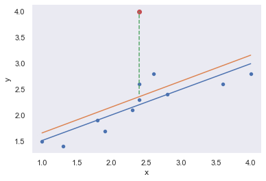
Fig. 17.5 An illustration of outliers. The orange line plots the regression line estimated when the anomalous (red) data point is included, and the dotted line shows the residual for the outlier. The blue line shows the regression line that would have been estimated without the anomalous observation included. The outlier has an unusual value on the outcome (y axis location) but not the predictor (x axis location), and lies a long way from the regression line. 
The second way in which an observation can be unusual is if it has high leverage: this happens when the observation is very different from all the other observations. This doesn’t necessarily have to correspond to a large residual: if the observation happens to be unusual on all variables in precisely the same way, it can actually lie very close to the regression line. An example of this is shown in panel A of Fig. 17.6 . The leverage of an observation is operationalised in terms of its hat value, usually written \(h_i\) . The formula for the hat value is rather complicated9 but its interpretation is not: \(h_i\) is a measure of the extent to which the \(i\) -th observation is “in control” of where the regression line ends up going. We won’t bother extracting the hat values here, but if you want to do this, you can use the get_influence method from the statsmodels.api package to inspect the relative influence of data points. For now, it is enough to get an intuitive, visual idea of what leverage can mean.
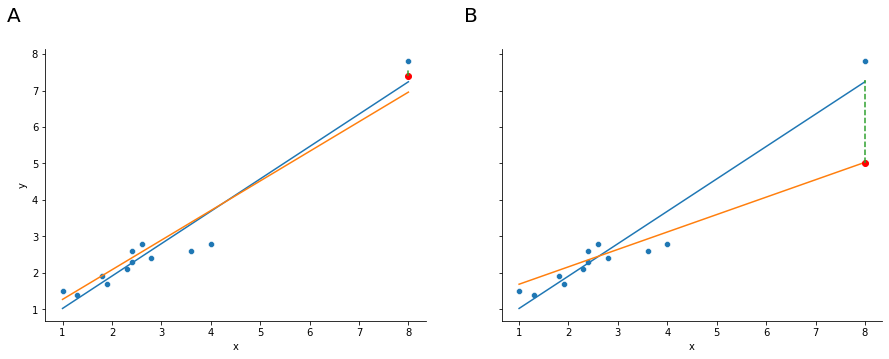
Fig. 17.6 Outliers showing high leverage points (panel A) and high influence points (panel B). 
In general, if an observation lies far away from the other ones in terms of the predictor variables, it will have a large hat value (as a rough guide, high leverage is when the hat value is more than 2-3 times the average; and note that the sum of the hat values is constrained to be equal to \(K+1\) ). High leverage points are also worth looking at in more detail, but they’re much less likely to be a cause for concern unless they are also outliers.
This brings us to our third measure of unusualness, the influence of an observation. A high influence observation is an outlier that has high leverage. That is, it is an observation that is very different to all the other ones in some respect, and also lies a long way from the regression line. This is illustrated in Fig. 17.6 , panel B. Notice the contrast to panel A, and to Fig. 17.5 : outliers don’t move the regression line much, and neither do high leverage points. But something that is an outlier and has high leverage… that has a big effect on the regression line.
That’s why we call these points high influence; and it’s why they’re the biggest worry. We operationalise influence in terms of a measure known as Cook’s distance,
Notice that this is a multiplication of something that measures the outlier-ness of the observation (the bit on the left), and something that measures the leverage of the observation (the bit on the right). In other words, in order to have a large Cook’s distance, an observation must be a fairly substantial outlier and have high leverage.
Again, if you want to quantify Cook’s distance, this can be done using using statsmodels.api . I won’t go through this in detail, but if you are interested, you can click to show the code, and see how I got the Cook’s distance values from statmodels .
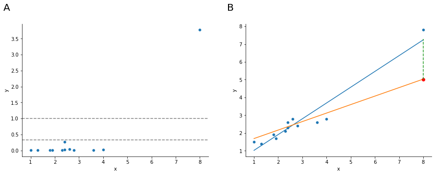
Fig. 17.7 A visualization of Cook’s distance as a means for identifying the influence of each data point. Panel B is the same as panel B in :numre:`fig-leverage-influence` above. The red dot show the effect on the entire regression line that sinking the final point from 7.4 to 5 has. Panel A shows Cook’s distance for the data set in which the data point at x = 8 is 5 (the orange line). The dashed lines show two possible cutoff points for a “large” Cook’s distance: either 1 or 4/N, in which N is the number of data points. 
As a rough guide, Cook’s distance greater than 1 is often considered large (that’s what I typically use as a quick and dirty rule), though a quick scan of the internet and a few papers suggests that \(4/N\) has also been suggested as a possible rule of thumb. As the visualization in :numre:`fig-cooks` illustrates, the red data point at x = 8 has a large Cook’s distance.
An obvious question to ask next is, if you do have large values of Cook’s distance, what should you do? As always, there’s no hard and fast rules. Probably the first thing to do is to try running the regression with that point excluded and see what happens to the model performance and to the regression coefficients. If they really are substantially different, it’s time to start digging into your data set and your notes that you no doubt were scribbling as your ran your study; try to figure out why the point is so different. If you start to become convinced that this one data point is badly distorting your results, you might consider excluding it, but that’s less than ideal unless you have a solid explanation for why this particular case is qualitatively different from the others and therefore deserves to be handled separately.[^noterobust] To give an example, let’s delete the observation from day 64, the observation with the largest Cook’s distance for the mod2 model, where we predicted my grumpiness on the basis of my sleep, and my baby’s sleep.
[^noterobust] An alternative is to run a "robust regression"; I might discuss robust regression in a later version of this book.
First, let’s get back to the original sleep data, and remind ourselves of what our model coefficients looked like:
| names | coef | se | T | pval | r2 | adj_r2 | CI[2.5%] | CI[97.5%] | |
|---|---|---|---|---|---|---|---|---|---|
| 0 | Intercept | 125.97 | 3.04 | 41.42 | 0.00 | 0.82 | 0.81 | 119.93 | 132.00 |
| 1 | dan_sleep | -8.95 | 0.55 | -16.17 | 0.00 | 0.82 | 0.81 | -10.05 | -7.85 |
| 2 | baby_sleep | 0.01 | 0.27 | 0.04 | 0.97 | 0.82 | 0.81 | -0.53 | 0.55 |
Then, we can remove the data from day 64, using the drop() method from pandas . Remember, as always, it’s Python, and Python is zero-indexed, so it starts counting the days at 0 and not 1, and that means that day 64 is on row 63!