Как читать ящик с усами python

Как читать ящик с усами python

Box Plot is the visual representation of the depicting groups of numerical data through their quartiles. Boxplot is also used for detect the outlier in data set. It captures the summary of the data efficiently with a simple box and whiskers and allows us to compare easily across groups. Boxplot summarizes a sample data using 25th, 50th and 75th percentiles. These percentiles are also known as the lower quartile, median and upper quartile.

A box plot consist of 5 things.

• Minimum
• First Quartile or 25%
• Median (Second Quartile) or 50%
• Third Quartile or 75%
• Maximum

To download the dataset used, click here.

Draw the box plot with Pandas:

One way to plot boxplot using pandas dataframe is to use boxplot() function that is part of pandas library.

Pandas Boxplots: Everything You Need to Know to Visualize Data

Data visualizations are a powerful tool to better understand the attributes of a data set.

pandas is a Python library built to streamline processes around capturing and manipulating relational data that has built-in methods for plotting and visualizing the values captured in its data structures.

One popular method for visualizing numerical data in pandas is the boxplot. In this post, you’ll learn the basics of a boxplot and see examples of boxplots in pandas.

Seaborn Boxplot — Tutorial and Examples

Seaborn is one of the most widely used data visualization libraries in Python, as an extension to Matplotlib. It offers a simple, intuitive, yet highly customizable API for data visualization.

In this tutorial, we'll take a look at how to plot a boxplot in Seaborn.

Boxplots are used to visualize summary statistics of a dataset, displaying attributes of the distribution like the data’s range and distribution.

Import Data

We’ll need to select a dataset with continuous features in order to create a boxplot, because boxplots display summary statistics for continuous variables — the median and range of a dataset. We’ll be working with the Forest Fires dataset.

We’ll begin with importing Pandas to load and parse the dataset. We’ll obviously want to import Seaborn as well. Finally, we’ll import the Pyplot module from Matplotlib, so that we can show the visualizations:

Let's use Pandas to read the CSV file and check how our DataFrame looks by printing its head. Additionally, we'll want to check if the dataset contains any missing values:

The second print statement returns False , which means that there isn't any missing data. If there were, we'd have to handle missing DataFrame values.

After we check for the consistency of our dataset, we want to select the continuous features that we want to visualize. We’ll save these as their own variables for convenience:

Plotting a Boxplot in Seaborn

Now that we have loaded in the data and selected the features that we want to visualize, we can create the Boxplots!

We can create the boxplot just by using Seaborn’s boxplot function. We pass in the dataframe as well as the variables we want to visualize:

If we want to visualize just the distribution of a categorical variable, we can provide our chosen variable as the x argument. If we do this, Seaborn will calculate the values on the Y-axis automatically, as we can see on the previous image.

However, if there’s a specific distribution that we want to see segmented by type, we can also provide a categorical X-variable and a continuous Y-variable.

This time around, we can see a boxplot generated for each day in the week, as specified in the dataset.

If we want to visualize multiple columns at the same time, what do we provide to the x and y arguments? Well, we provide the labels for the data we want, and provide the actual data using the data argument.

We can create a new DataFrame containing just the data we want to visualize, and melt() it into the data argument, providing labels such as x='variable' and y='value' :

Free eBook: Git Essentials

Check out our hands-on, practical guide to learning Git, with best-practices, industry-accepted standards, and included cheat sheet. Stop Googling Git commands and actually learn it!

Customize a Seaborn Boxplot

Change Boxplot Colors

Seaborn will automatically assign the different colors to different variables so we can easily visually differentiate them. Though, we can also supply a list of colors to be used if we'd like to specify them.

After choosing a list of colors with hex values (or any valid Matplotlib color), we can pass them into the palette argument:

Customize Axis Labels

We can adjust the X-axis and Y-axis labels easily using Seaborn, such as changing the font size, changing the labels, or rotating them to make the ticks easier to read:

Ordering Boxplots

If we want to view the boxes in a specific order, we can do that by making use of the order argument, and supplying the column names in the order you want to see them in:

Creating Subplots

If we wanted to separate out the plots for the individual features into their own subplots, we could do that by creating a figure and axes with the subplots function from Matplotlib. Then, we use the axes object and access them via their index. The boxplot() function accepts an ax argument, specifying on which axes it should be plotted on:

Boxplot with Data Points

We could even overlay a swarmplot onto the boxplot in order to see the distribution and samples of the points comprising that distribution, with a bit more detail.

In order to do this, we just create a single figure object and then create two different plots. The stripplot() will be overlaid over the boxplot() , since they're on the same axes / figure :

Conclusion

In this tutorial, we've gone over several ways to plot a boxplot using Seaborn and Python. We've also covered how to customize the colors, labels, ordering, as well as overlay swarmplots and subplot multiple boxplots.

If you're interested in Data Visualization and don't know where to start, make sure to check out our bundle of books on Data Visualization in Python:

Data Visualization in Python

Become dangerous with Data Visualization

✅ 30-day no-question money-back guarantee

✅ Beginner to Advanced

✅ Updated regularly for free (latest update in April 2021)

✅ Updated with bonus resources and guides

Data Visualization in Python with Matplotlib and Pandas is a book designed to take absolute beginners to Pandas and Matplotlib, with basic Python knowledge, and allow them to build a strong foundation for advanced work with these libraries — from simple plots to animated 3D plots with interactive buttons.

It serves as an in-depth guide that'll teach you everything you need to know about Pandas and Matplotlib, including how to construct plot types that aren't built into the library itself.

Data Visualization in Python, a book for beginner to intermediate Python developers, guides you through simple data manipulation with Pandas, covers core plotting libraries like Matplotlib and Seaborn, and shows you how to take advantage of declarative and experimental libraries like Altair. More specifically, over the span of 11 chapters this book covers 9 Python libraries: Pandas, Matplotlib, Seaborn, Bokeh, Altair, Plotly, GGPlot, GeoPandas, and VisPy.

It serves as a unique, practical guide to Data Visualization, in a plethora of tools you might use in your career.

Seaborn Boxplot – How to Create Box and Whisker Plots

In this tutorial, you’ll learn how to use Seaborn to create a boxplot (or a box and whisker plot). Boxplots are important plots that allow you to easily understand the distribution of your data in a meaningful way. Boxplots allow you to understand the attributes of a dataset, including its range and distribution.

By the end of this tutorial, you’ll have learned:

• What boxplots are and how they can be interpreted
• How to create a basic boxplot in Seaborn
• How to add multiple columns and rows to a boxplot
• How to style a boxplot in Seaborn
• How to order and rotate your Seaborn boxplot

Check out the sections below If you’re interested in something specific. If you want to learn more about Seaborn, check out my other Seaborn tutorials, like the bar chart tutorial or line chart tutorial.

Table of Contents

What is a boxplot?

Boxplots are helpful charts that clearly illustrate the distribution in a dataset, by visualizing the range, distribution, and extreme values. A boxplot is a helpful data visualization that illustrates five different summary statistics for your data. It helps you understand the data in a much clearer way than just seeing a single summary statistic.

Specifically, boxplots show a five-number summary that includes:

• the minimum,
• the first quartile (25th percentile),
• the median,
• the third quartile (75th percentile),
• the maximum

Additionally, boxplots will identify any outliers that exist in the data. Outliers are generally classified as being outside 1.5 times the interquartile range.

This post is part of the Seaborn learning path! The learning path will take you from a beginner in Seaborn to creating beautiful, customized visualizations. Check it out now!

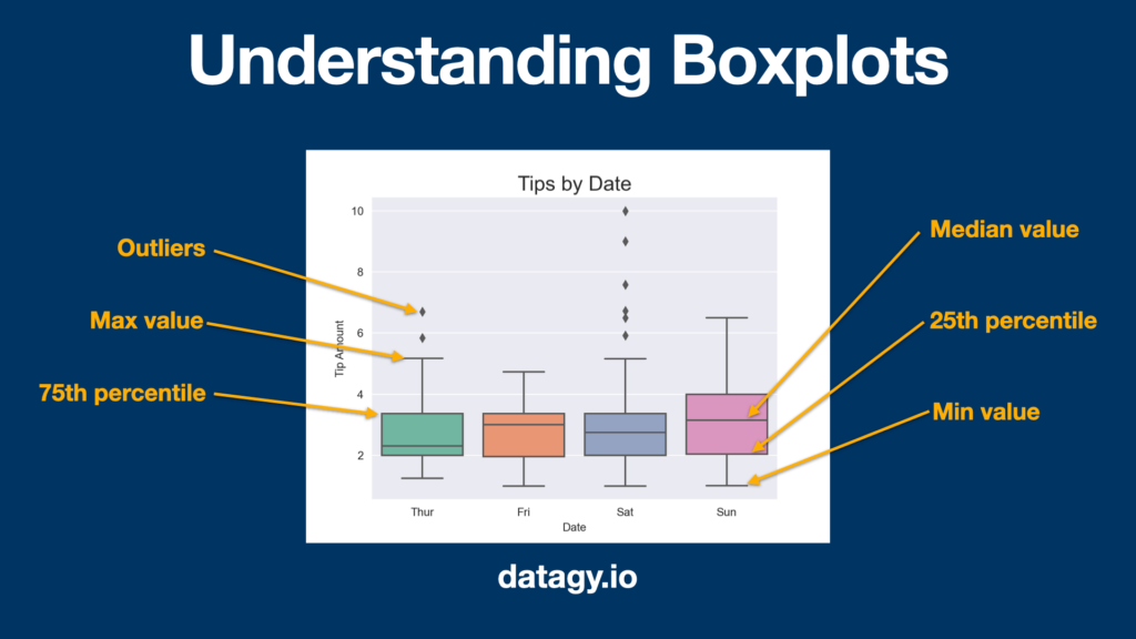
The median line can be very descriptive as well. If the line is higher in the interquartile range (the box), the data is said to be negatively skewed. Inversely, if the median line is lower in the box, the data is said to be positively skewed.

Understanding the Seaborn Boxplot Function

Before diving into creating boxplots with Seaborn, let’s take a look at the function itself and the different parameters that it offers. This can be an important first step that allows you to better understand what can be done with the function and how you can customize your code:

Let’s break down what each of these parameters does:

• x=None represents the data to use for the x-axis
• y=None represents the data to use for the y-axis
• hue=None represents the data to use to break your data by break
• data=None represents the DataFrame to use for your data
• order=None represents how to order your data
• hue_order=None similar to order , represents how to order your data
• orient=None indicates whether data should be horizontal or vertical
• color=None represents the color(s) to use
• palette=None represents the pallette to use
• saturation=0.75 represents the saturation of the color
• width=0.8 represents the width of an element
• dodge=True represents when hue nesting is used, how to shift categorical data
• fliersize=5 represents the size of the markers for outliers
• linewidth=None represents the width of the lines in the graph
• whis=1.5 represents the proportion of the interquartile range to extend the plot whiskers
• ax=None represents the axes object to draw on

Loading a Sample Dataset

To follow along with this tutorial, let’s load a sample dataset that we can use throughout this tutorial. Seaborn comes with a number of built-in datasets, including a valuable tips dataset that shows tips given to restaurant workers.

Let’s load the dataset using the Seaborn load_dataset() function and take a quick look at it:

Now that we have a dataset loaded, let’s dive into how to use Seaborn to create a boxplot.

How to Create a Boxplot in Seaborn

Creating a boxplot in Seaborn is made easy by using the sns.boxplot() function. Let’s start by creating a boxplot that breaks the data out by day column on the x-axis and shows the total_bill column on the y-axis. Let’s see how we’d do this in Python:

This returns the following image:

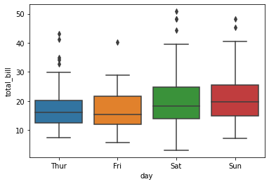
We can see that by using just two lines of code, we were able to create and display a boxplot! Because Seaborn is designed to handle Pandas DataFrames easily, we can simply refer to the column names directly, as long as we pass the DataFrame into the data parameter.

By default, the styling of a Seaborn boxplot is a little uninspiring. In the following section, you’ll learn how to modify the styling of your plot.

Styling a Seaborn boxplot

Seaborn makes it easy to apply a style and a color palette to our visualizations. This can be done using the set_style() and set_palette() functions, respectively.

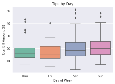
Let’s learn how we can apply some style and a different color palette to the Seaborn boxplot. Let’s apply the ‘darkgrid’ style and the ‘Set2’ palette to our visualization:

This returns a much nicer-looking visualization, as shown below:

Let’s break down exactly what we did in our code:

1. We used the sns.set_style() function to apply the ‘darkgrid’ style
2. We then applied the ‘Set2’ palette to apply a muted color-scheme to our visualizations.

Both of these changes were made globally, meaning that any subsequent visualizations would have these changes applied as well.

In the following section, you’ll learn how to add titles and modify axis labels in a Seaborn boxplot.

Adding titles and axis labels to Seaborn boxplots

In this section, you’ll learn how to add a title and descriptive axis labels to your Seaborn boxplot. By default, Seaborn will attempt to infer the axis titles by using the column names. This may not always be what you want, especially when you want to add something like unit labels.

Because Seaborn is built on top of Matplotlib, you can use the pyplot module to add titles and axis labels. S

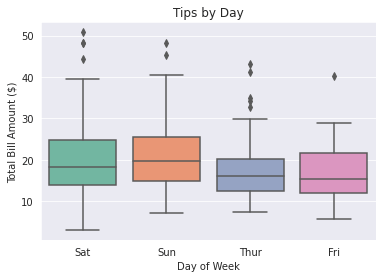
We can also use Matplotlib to add some descriptive titles and axis labels to our plot to help guide the interpretation of the data even further. Let’s now add a descriptive title and some axis labels that aren’t based on the dataset.

This returns our chart, with a helpful title and some axis labels added. Matplotlib gives you a lot of control over how you add titles and axis labels.

How to Change the Order of Seaborn Boxplots

The Seaborn boxplot() function gives you significant control over how you order items in the plot. Because Seaborn will, by default, try to order items numerically or alphabetically, you may end up with unexpected results.

In our earlier example, There may be times when you want to sort your data in different ways. Currently, Seaborn is inferring the order us, but we can also specify a particular order.

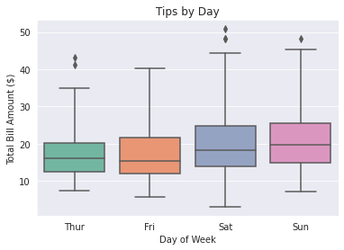
To do this, we use the order= parameter. For example, if we wanted to place the weekend days first, we could write:

In the code above, we passed in a list of items to the order= parameter. This allowed us to override the default behavior to define a custom sorting order. This returns our updated boxplot:

How to Rotate a Seaborn Boxplot

In some cases, your data will be easier to understand if it is in a horizontal format. This can be particularly true when you’re dealing with a large number of variables and want to be able to easily scan down the data.

By default, Seaborn will infer the orientation of your boxplot based on the data that exists in the dataset. Seaborn provides two different methods to do this. If both your variables are numerical (or if you’re using a wide-dataset) you can specify orient=’h’ to display your data in a horizontal format.

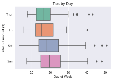
Alternatively, if you’re not plotting two numerical variables, you can simply flip the x= and y= parameters. Let’s see how we can do this in Python:

This returns the following boxplot:

In the following section, you’ll learn how to change the whisker length in a boxplot.

Changing Whisker Length in Seaborn Boxplot

By default, Seaborn boxplots will use a whisker length of 1.5. What this means, is that values that sit outside of 1.5 times the interquartile range (in either a positive or negative direction) from the lower and upper bounds of the box.

Seaborn provides two different methods for changing the whisker length:

1. Changing the proportion which determine outliers, and
2. Setting upper and lower percentile bounds to capture data

Setting Interquartile Range Proportion in Seaborn Boxplots

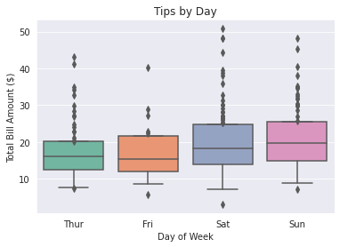
Say we wanted to include data points that exist within the range of two times the interquartile range, we can specify the whis= parameter.

Let’s try this in Python:

This returns the following boxplot:

In the code sample above, we increased the range of the whiskers to include values that fall within 2 times the interquartile range.

In the following section, you’ll learn how to set percentile limits on Seaborn boxplot whiskers.

Setting Percentile Limits on Seaborn Boxplot Whiskers

There may be times when you want to set upper and lower limits on the percentages of data points to include.

For example, if you wanted to include everything except for the bottom and top 5% of your data within the box and whiskers, you could write:

This returns the following boxplot:

How to Create a Grouped Seaborn Boxplot

Seaborn makes it easy to add another dimension to our boxplots, using the hue= parameter. In the example we have been using, it may be helpful to split the data also by gender to see how the data differs based on different genders.

We can do this, similar to other Seaborn plots, using the hue= parameter. Let’s add this to our plot to see how this changes the plot:

This returns the following image:

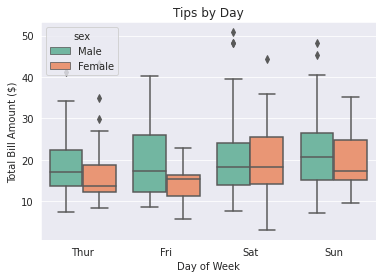
This allows us to see how the spread of data differs, not only by the day of the week but also by gender.

Conclusion

In this post, you learned what a boxplot is and how to create a boxplot in Seaborn. Specially, you learned how to customize the plot using styles and palettes, adding a title and axis labels to the chart, as well as modifying different data elements within the chart. Finally, you learned how to plot a second dimension to create a grouped boxplot.