Cv2 threshold python что делает
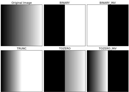
Result is given below :
Adaptive Thresholding
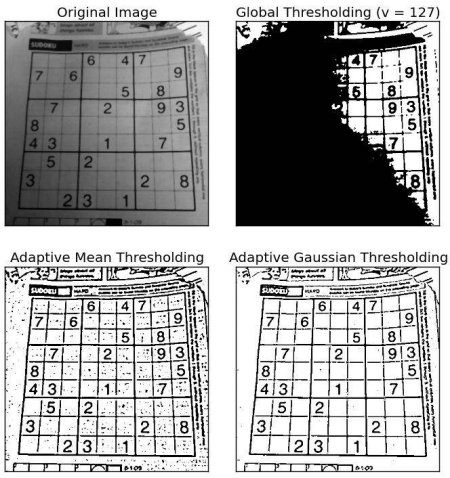
In the previous section, we used a global value as threshold value. But it may not be good in all the conditions where image has different lighting conditions in different areas. In that case, we go for adaptive thresholding. In this, the algorithm calculate the threshold for a small regions of the image. So we get different thresholds for different regions of the same image and it gives us better results for images with varying illumination.
It has three ‘special’ input params and only one output argument.
Adaptive Method — It decides how thresholding value is calculated.
- cv2.ADAPTIVE_THRESH_MEAN_C : threshold value is the mean of neighbourhood area.
- cv2.ADAPTIVE_THRESH_GAUSSIAN_C : threshold value is the weighted sum of neighbourhood values where weights are a gaussian window.
Block Size — It decides the size of neighbourhood area.
C — It is just a constant which is subtracted from the mean or weighted mean calculated.
Below piece of code compares global thresholding and adaptive thresholding for an image with varying illumination:
Otsu’s Binarization
In the first section, I told you there is a second parameter retVal. Its use comes when we go for Otsu’s Binarization. So what is it?
In global thresholding, we used an arbitrary value for threshold value, right? So, how can we know a value we selected is good or not? Answer is, trial and error method. But consider a bimodal image (In simple words, bimodal image is an image whose histogram has two peaks). For that image, we can approximately take a value in the middle of those peaks as threshold value, right ? That is what Otsu binarization does. So in simple words, it automatically calculates a threshold value from image histogram for a bimodal image. (For images which are not bimodal, binarization won’t be accurate.)
For this, our cv2.threshold() function is used, but pass an extra flag, cv2.THRESH_OTSU. For threshold value, simply pass zero. Then the algorithm finds the optimal threshold value and returns you as the second output, retVal. If Otsu thresholding is not used, retVal is same as the threshold value you used.
Check out below example. Input image is a noisy image. In first case, I applied global thresholding for a value of 127. In second case, I applied Otsu’s thresholding directly. In third case, I filtered image with a 5×5 gaussian kernel to remove the noise, then applied Otsu thresholding. See how noise filtering improves the result.
What is Thresholding?

Thresholding is a process of dividing an image into two (or more) classes of pixels, i.e. “foreground” and “background”. It is mostly used in various Image processing tasks, such as eliminating noise in the OCR process which allows greater image recognition accuracy, segmentation etc.
In order to obtain a thresholded image, usually, we convert the original image into a grayscale image and then apply the thresholding technique. This method is also known as Binarization as we convert the image into a binarized form, i.e. if the value of a pixel is lesser than the threshold value, convert it to 0(Black). If the value of a pixel is greater than the threshold value, convert it to 1(White) or vice-versa.
Let’s understand the importance of binarization with an example on OCR:
NOTE: For all my examples I am using pytesseract (a wrapper for google’s tesseract), Matplotlib and OpenCV.
Therefore please install all the above-mentioned libraries. For me, as I was working on a Colab Notebook, I need to install the pytesseract only.
And import them.
Okay, now suppose you have an image like below and you have to detect the text in it-
First, read the Image file, please make sure it is supported by OpenCV and then pass the object of this image to the image_to_string function as follows
As you can see the code has detected the right text. But will it perform the same on a noisy image like below?
Clearly, the output is not what you might have expected. let’s try the binary thresholding technique and then check the result.
From the above result, you might get the clue, why the threshold techniques are important in digital image processing tasks.
Simple Thresholding
If the pixel value is greater than a threshold value, it is assigned one value (maybe white), else it is assigned another value (maybe black). The function used is
- The first argument is the source image(grayscale image).
- The second argument is the threshold value which is used to classify the pixel values.
- The third argument is the maxVal which represents the value to be given if the pixel value is more than (sometimes less than) the threshold value.
- The fourth argument is the style of thresholding. OpenCV provides different styles of thresholding. Check the Documentation page.
Note:- Although we get the correct text for that image using simple threshold, however, this may not be the case with some other image. There we need to change the threshold value as accordingly or we need to perform some more operations to get the correct result.
Apart from the simple threshold, OpenCV provides more functions for thresholding such as Adaptive thresholding and Otsu’s Binarization.
Let’s check another example:-
Following is an image of a Shopfront.
First, open the image in grayscale mode and test the tesseract
Unfortunately, for this image, it didn’t output any text. So what went wrong?
It looks like the background cover more area than the texts, Let’s crop that particular area and then test again.
Again we can see that the result is not accurate, it didn’t detect ‘FOOD’ written at the bottom right of the image. Now this time I will try the Adaptive threshold. Following is the syntax for it.
Adaptive threshold
In this, the algorithm calculates the threshold for small regions of the image. So we get different thresholds for different regions of the same image and it gives us better results for images with varying illumination.
Though the code produces the correct text, yet it interprets noises as Characters as well. To overcome this, we need to blur the image a little bit and then test again.
Image blurring is achieved by convolving the image with a normalized box filter. It simply takes the average of all the pixels under the kernel area and replaces the central element with this average. This is done by the function cv2.blur(). It is useful for removing noise in the image. Blurring is a separate topic in itself, so I will cover it later in another post.
Conclusion
Image Thresholding is one of the most commonly used technique in many image processing tasks. However, we have to keep in mind that for perfect segmentation we need to try different threshold values.
Note:- Thresholding gives better results if the image is of higher contrast. Try to change the contrast value of the pixels and then apply the threshold.
In the end, I want you to try this by yourself and see what results you’ll get with different images. You can try to find other texts in the Shopfront image or try this image and share your reviews. Are you able to find the text in the image?
Hint: Try cv2.THRESH_BINARY in cv2.threshold() with thresh value = 1
For more details please check out this link and Notebook, it has an in-depth analysis of various thresholding techniques that you can also apply. Thanks to Ankit Kumar Singh for sharing his Notebook with us.
Image Thresholding
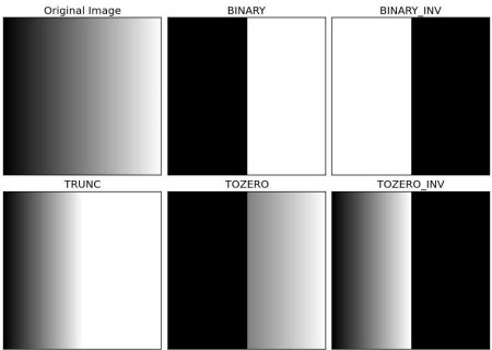
Here, the matter is straight forward. If pixel value is greater than a threshold value, it is assigned one value (may be white), else it is assigned another value (may be black). The function used is cv2.threshold. First argument is the source image, which should be a grayscale image. Second argument is the threshold value which is used to classify the pixel values. Third argument is the maxVal which represents the value to be given if pixel value is more than (sometimes less than) the threshold value. OpenCV provides different styles of thresholding and it is decided by the fourth parameter of the function. Different types are:
- cv2.THRESH_BINARY
- cv2.THRESH_BINARY_INV
- cv2.THRESH_TRUNC
- cv2.THRESH_TOZERO
- cv2.THRESH_TOZERO_INV
Documentation clearly explain what each type is meant for. Please check out the documentation.
Two outputs are obtained. First one is a retval which will be explained later. Second output is our thresholded image.
To plot multiple images, we have used plt.subplot() function. Please checkout Matplotlib docs for more details.
Result is given below :
Adaptive Thresholding
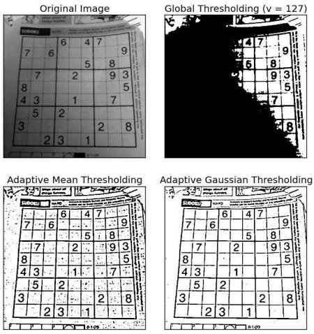
In the previous section, we used a global value as threshold value. But it may not be good in all the conditions where image has different lighting conditions in different areas. In that case, we go for adaptive thresholding. In this, the algorithm calculate the threshold for a small regions of the image. So we get different thresholds for different regions of the same image and it gives us better results for images with varying illumination.
It has three ‘special’ input params and only one output argument.
- cv2.ADAPTIVE_THRESH_MEAN_C : threshold value is the mean of neighbourhood area.
- cv2.ADAPTIVE_THRESH_GAUSSIAN_C : threshold value is the weighted sum of neighbourhood values where weights are a gaussian window.
Block Size — It decides the size of neighbourhood area.
C — It is just a constant which is subtracted from the mean or weighted mean calculated.
Below piece of code compares global thresholding and adaptive thresholding for an image with varying illumination:
Otsu’s Binarization
In the first section, I told you there is a second parameter retVal. Its use comes when we go for Otsu’s Binarization. So what is it?
In global thresholding, we used an arbitrary value for threshold value, right? So, how can we know a value we selected is good or not? Answer is, trial and error method. But consider a bimodal image (In simple words, bimodal image is an image whose histogram has two peaks). For that image, we can approximately take a value in the middle of those peaks as threshold value, right ? That is what Otsu binarization does. So in simple words, it automatically calculates a threshold value from image histogram for a bimodal image. (For images which are not bimodal, binarization won’t be accurate.)
For this, our cv2.threshold() function is used, but pass an extra flag, cv2.THRESH_OTSU . For threshold value, simply pass zero. Then the algorithm finds the optimal threshold value and returns you as the second output, retVal . If Otsu thresholding is not used, retVal is same as the threshold value you used.
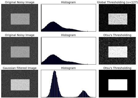
Check out below example. Input image is a noisy image. In first case, I applied global thresholding for a value of 127. In second case, I applied Otsu’s thresholding directly. In third case, I filtered image with a 5×5 gaussian kernel to remove the noise, then applied Otsu thresholding. See how noise filtering improves the result.
How Otsu’s Binarization Works?
This section demonstrates a Python implementation of Otsu’s binarization to show how it works actually. If you are not interested, you can skip this.
Since we are working with bimodal images, Otsu’s algorithm tries to find a threshold value (t) which minimizes the weighted within-class variance given by the relation :

![q_1(t) = \sum_<i=1>^ <t>P(i) \quad \& \quad q_1(t) = \sum_<i=t+1>^ <I>P(i) \mu_1(t) = \sum_<i=1>^ <t>\frac<iP(i)> <q_1(t)>\quad \& \quad \mu_2(t) = \sum_<i=t+1>^ <I>\frac<iP(i)> <q_2(t)>\sigma_1^2(t) = \sum_<i=1>^ <t>[i-\mu_1(t)]^2 \frac<P(i)> <q_1(t)>\quad \& \quad \sigma_2^2(t) = \sum_<i=t+1>^ <I>[i-\mu_1(t)]^2 \frac<P(i)><q_2(t)>» /></p>
<p>It actually finds a value of t which lies in between two peaks such that variances to both classes are minimum. It can be simply implemented in Python as follows:</p>
<p><em>(Some of the functions may be new here, but we will cover them in coming chapters)</em></p>
<h2>OpenCV Thresholding in Python with cv2.threshold()</h2>
<p><img decoding=](https://opencv24-python-tutorials.readthedocs.io/en/latest/_images/math/588a446d9a466ac81104cf588afec8ec9d713ffe.png)
Thresholding is a simple and efficient technique to perform basic segmentation in an image, and to binarize it (turn it into a binary image) where pixels are either 0 or 1 (or 255 if you're using integers to represent them).
Typically, you can use thresholding to perform simple background-foreground segmentation in an image, and it boils down to variants on a simple technique for each pixel:
This essential process is known as Binary Thresholding. Now — there are various ways you can tweak this general idea, including inverting the operations (switching the > sign with a < sign), setting the pixel_value to the threshold instead of a maximum value/0 (known as truncating), keeping the pixel_value itself if it's above the threshold or if it's below the threshold .
All of these have conveniently been implemented in OpenCV as:
- cv2.THRESH_BINARY
- cv2.THRESH_BINARY_INV
- cv2.THRESH_TRUNC
- cv2.THRESH_TOZERO
- cv2.THRESH_TOZERO_INV
. respectively. These are relatively "naive" methods in that hey're fairly simple, don't account for context in images, have knowledge of what shapes are common, etc. For these properties — we'd have to employ much more computationally expensive and powerful techniques.
Advice: If you'd like to learn more about multi-class semantic segmentation with Deep Learning — you can enroll our DeepLabV3+ Semantic Segmentation with Keras!
Now, even with the "naive" methods — some heuristics can be put into place, for finding good thresholds, and these include the Otsu method and the Triangle method:
- cv2.THRESH_OTSU
- cv2.THRESH_TRIANGLE
Note: OpenCV thresholding is a rudimentary technique, and is sensitive to lighting changes and gradients, color heterogeneity, etc. It's best applied on relatively clean pictures, after blurring them to reduce noise, without much color variance in the objects you want to segment.
Another way to overcome some of the issues with basic thresholding with a single threshold value is to use adaptive thresholding which applies a threshold value on each small region in an image, rather than globally.
Simple Thresholding with OpenCV
Thresholding in OpenCV's Python API is done via the cv2.threshold() method — which accepts an image (NumPy array, represented with integers), the threshold, maximum value and thresholding method (how the threshold and maximum_value are used):
The return code is just the applied threshold:
Here, since the threshold is 220 and we've used the THRESH_BINARY method — every pixel value above 220 will be increased to 255 , while every pixel value below 220 will be lowered to 0 , creating a black and white image, with a "mask", covering the foreground objects.
Why 220? Knowing what the image looks like allows you to make some approximate guesses about what threshold you can choose. In practice, you'll rarely want to set a manual threshold, and we'll cover automatic threshold selection in a moment.
Let's plot the result! OpenCV windows can be a bit finicky, so we'll plot the original image, blurred image and results using Matplotlib:
Thresholding Methods
As mentioned earlier, there are various ways you can use the threshold and maximum value in a function. We've taken a look at the binary threshold initially. Let's create a list of methods, and apply them one by one, plotting the results:
THRESH_BINARY and THRESH_BINARY_INV are inverse of each other, and binarize an image between 0 and 255 , assigning them to the background and foreground respectively, and vice versa.
THRESH_TRUNC binarizes the image between threshold and 255 .
THRESH_TOZERO and THRESH_TOZERO_INV binarize between 0 and the current pixel value ( src(x, y) ). Let's take a look at the resulting images:


Free eBook: Git Essentials
Check out our hands-on, practical guide to learning Git, with best-practices, industry-accepted standards, and included cheat sheet. Stop Googling Git commands and actually learn it!
These methods are intuitive enough — but, how can we automate a good threshold value, and what does a "good threshold" value even mean? Most of the results so far had non-ideal masks, with marks and specks in them. This happens because of the difference in the reflective surfaces of the coins — they're not uniformly colored due to the difference in how ridges reflect light.
We can, to a degree, battle this by finding a better global threshold.
Automatic/Optimized Thresholding with OpenCV
OpenCV employs two effective global threshold searching methods — Otsu's method, and the Triangle method.
Otsu's method assumes that it's working on bi-modal images. Bi-modal images are images whose color histograms only contain two peaks (i.e. has only two distinct pixel values). Considering that the peaks each belong to a class such as a "background" and "foreground" — the ideal threshold is right in the middle of them.
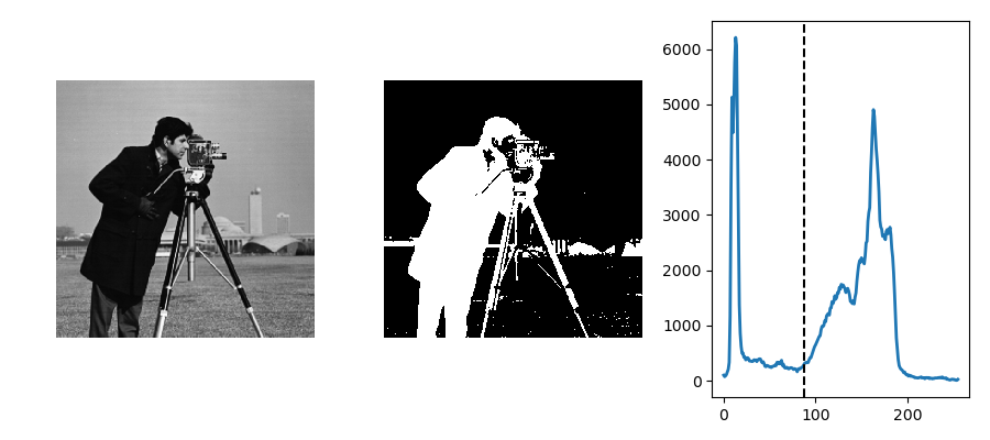
Image credit: https://scipy-lectures.org/
You can make some images more bi-modal with gaussian blurs, but not all.
An alternative algorithm is the triangle algorithm, which calculates the distance between the maximum and minimum of the grey-level histogram and draws a line. The point at which that line is maximally far away from the rest of the histogram is chosen as the treshold:
There's no competition between them — they each work on different types of images, so it's best to try them out and see which returns the better result. Both of these assume a greyscaled image, so we'll need to convert the input image to gray via cv2.cvtColor() :
Let's run the image through with both methods and visualize the results:
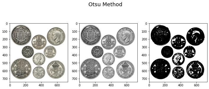
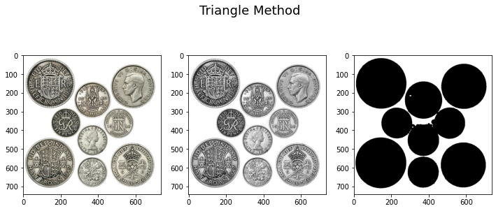
Here, the triangle method outperforms Otsu's method, because the image isn't bi-modal:
However, it's clear how the triangle method was able to work with the image and produce a more satisfying result.
Limitations of OpenCV Thresholding
Thresholding with OpenCV is simple, easy and efficient. Yet, it's fairly limited. As soon as you introduce colorful elements, non-uniform backgrounds and changing lighting conditions — global thresholding as a concept becomes too rigid.
Images are usually too complex for a single threshold to be enough, and this can partially be addressed through adaptive thresholding, where many local thresholds are applied instead of a single global one. While also limited, adaptive thresholding is much more flexible than global thresholding.
Conclusion
In recent years, binary segmentation (like what we did here) and multi-label segmentation (where you can have an arbitrary number of classes encoded) has been successfully modeled with deep learning networks, which are much more powerful and flexible. In addition, they can encode global and local context into the images they're segmenting. The downside is — you need data to train them, as well as time and expertise.
For on-the-fly, simple thresholding, you can use OpenCV. For accurate, production-level segmentation, you'll want to use neural networks.
Going Further — Practical Deep Learning for Computer Vision
Your inquisitive nature makes you want to go further? We recommend checking out our Course: "Practical Deep Learning for Computer Vision with Python".
Another Computer Vision Course?
We won't be doing classification of MNIST digits or MNIST fashion. They served their part a long time ago. Too many learning resources are focusing on basic datasets and basic architectures before letting advanced black-box architectures shoulder the burden of performance.
We want to focus on demystification, practicality, understanding, intuition and real projects. Want to learn how you can make a difference? We'll take you on a ride from the way our brains process images to writing a research-grade deep learning classifier for breast cancer to deep learning networks that "hallucinate", teaching you the principles and theory through practical work, equipping you with the know-how and tools to become an expert at applying deep learning to solve computer vision.