Как исправить ошибку #VALUE! ошибка

Значение! ошибка появляется, когда значение не соответствует ожидаемому типу. Это может произойти, когда ячейки оставлены пустыми, когда функции, ожидающей число, присваивается текстовое значение и когда даты обрабатываются Excel как текст. Исправление ошибки #VALUE! ошибка обычно просто вопрос ввода правильного значения. См. Ниже дополнительную информацию и примеры.
Объяснение
Значение! ошибка появляется, когда значение не соответствует ожидаемому типу. Это может произойти, когда ячейки оставлены пустыми, когда функции, ожидающей число, присваивается текстовое значение и когда даты оцениваются Excel как текст. Исправление ошибки #VALUE! ошибка обычно просто вопрос ввода правильного значения.
Ошибка #VALUE — это немного сложно, потому что некоторые функции автоматически игнорируют недопустимые данные. Например, функция СУММ просто игнорирует текстовые значения, но обычное сложение или вычитание с помощью оператора плюс (+) или минус (-) вернет #VALUE! ошибка, если какие-либо значения являются текстовыми.
В приведенных ниже примерах показаны формулы, возвращающие ошибку #VALUE, а также варианты устранения.
Пример # 1 — неожиданное текстовое значение
В приведенном ниже примере ячейка C3 содержит текст «NA», а F2 возвращает #VALUE! ошибка:

Один из вариантов исправления — ввести отсутствующее значение в C3. Тогда формула в F3 работает правильно:

Другой вариант в этом случае — переключиться на функцию СУММ. Функция СУММ автоматически игнорирует текстовые значения:

Пример # 2 — ошибочный пробел
Иногда ячейка с одним или несколькими ошибочными пробелами выдает #VALUE! ошибка, как показано на экране ниже:

Замечание C3 выглядит совершенно пустым. Однако, если выбран C3, можно увидеть, что курсор находится чуть правее одного пробела:

Excel возвращает #VALUE! ошибка, потому что пробел является текстом, так что на самом деле это просто еще один случай из Примера №1 выше. Чтобы исправить эту ошибку, убедитесь, что ячейка пуста, выбрав ячейку и нажав клавишу Delete.
Примечание: если у вас возникли проблемы с определением, действительно ли ячейка пуста, используйте для проверки функцию ISBLANK или LEN.
Пример # 3 — аргумент функции не ожидаемого типа
Значение! ошибка также может возникнуть, если аргументы функции не являются ожидаемыми типами. В приведенном ниже примере функция ЧИСТРАБДНИ настроена для расчета количества рабочих дней между двумя датами. В ячейке C3 «яблоко» не является допустимой датой, поэтому функция ЧИСТРАБДНИ не может вычислить рабочие дни и возвращает # ЗНАЧ! ошибка:

Ниже, когда правильная дата введена в C3, формула работает должным образом:

Пример # 4 — даты хранятся в виде текста
Иногда рабочий лист может содержать недопустимые даты, поскольку они хранятся в виде текста. В приведенном ниже примере функция EDATE используется для расчета срока годности через три месяца после даты покупки. Формула в C3 возвращает #VALUE! ошибка, потому что дата в B3 хранится как текст (т.е. не распознается должным образом как дата):

Когда дата в B3 зафиксирована, ошибка устранена:

Если вам нужно исправить много дат, сохраненных в виде текста, на этой странице представлены некоторые варианты исправления.
Excel VALUE Function – How To Use
The VALUE function is a text function that converts a number from text format to numerical format where data is in an Excel-recognized format such as date, currency, time, etc. Mostly, if Excel recognizes a number, it automatically converts the data into numerical format. However, in other cases, we can do so using the VALUE function.
The VALUE function is most helpful when we seek compatibility with other spreadsheet programs and for using the numerical text resulting from text functions in calculations.

Table of Contents
Syntax
The syntax of the VALUE function is quite straightforward and is given below.
Arguments:
The VALUE function accepts only one argument, and it is mandatory.
'text'– This mandatory argument contains the value in text format that needs to be converted. The value of the text argument can be passed as a direct value in double quotes or as a cell reference.
Important Characteristics of the VALUE Function
Some noteworthy features of the VALUE function are as follows.
- The VALUE function only accepts the value that is recognized by Microsoft Excel such as constant number, locale formatted number, date, or time. If the value of the text argument is any value that is not recognized by Excel, the function results in a #VALUE! error.
- If the value of the text argument is empty, the VALUE function returns zero.
When using the VALUE function, it is important to note the alignment of the data as left-aligned data indicates text format whereas right-aligned data is number format.
Examples of VALUE Function
There are instances when the given data which looks like a number cannot be used further for calculations and analysis. In such scenarios, the VALUE function comes in very handy. Below are some examples to provide a better understanding of the function.
Example 1 – Simple Use of VALUE Function
In this example, we will use different types of input values for the text argument to better understand the functionality of the VALUE function.
We have taken time, date, date and time together, number in text format, and percentage as the input values. The function used is as follows.
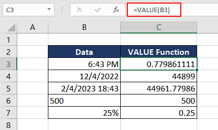
In the first example, the value of the text argument is a time value which upon conversion to numerical format is transformed into the serial number. Excel stores time as fractions of a day. The VALUE function simply converted the time format to an actual serial number which can further be used in formulas.
The next example is in date format and like the time data, the VALUE function converts the date value to a sequential number as stored in Excel. The third example is a combination of date and time, and the VALUE function returns the expected result of the corresponding serial number and fraction of both date and time in cell C5.
The fourth example is a text which looks like a number. If we wish to use the data in cell B6 for any calculations, the result will also take on the text format. With the help of the VALUE function, the number is transformed from text format to numerical format.
The last example is a percentage value. The VALUE function returns the calculated numerical value of the percentage which is 0.25 in this case.
Now that the basic functionality of the VALUE function is clear, check some useful applications of the same in the examples below.
Example 2 – Converting String to Number using VALUE Function
In this scenario, we collected small donations from our neighbors to get essentials for the homeless shelter. The data collected was user-generated hence it is in text format.
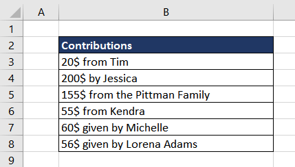
To calculate the total donations received, we can extract the dollar amount and then sum it up. To segregate the donation amount from the given text, we will use the TEXTBEFORE function. It will extract the characters that occur before the dollar sign ($), which is the amount in this case. The formula used is as follows.
Now that the donation amount is segregated in column C, the total donation can be calculated.
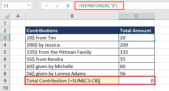
Unfortunately, all the extracted data in column C is text, which is clear due to its left alignment, since the TEXTBEFORE function is a text function. Therefore, the total sum couldn't be downloaded as seen in cell C10. To rectify this, we will use the VALUE function to convert all the data in column C into the numeric format and then calculate the total donation received. The updated formula to be used is as follows.
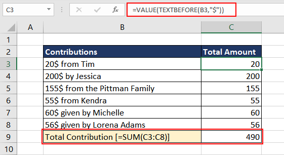
We can combine everything in one formula as follows.
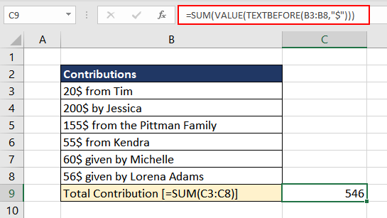
Note: One can also use the LEFT function in place of the TEXTBEFORE function to achieve the same result.
Example 3 – Converting Currency to Numerical Format
Here, in this case, we have received the monthly sales for the last year. As the sales report is from the India office, the currency formatting is different where a comma is used as a group separator in hundreds, thousands, and so on. Excel does not recognize the formatting, so it treats the sales numbers as text.
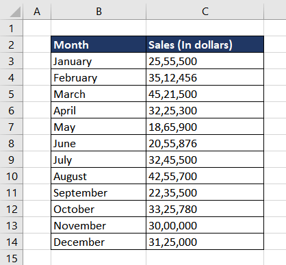
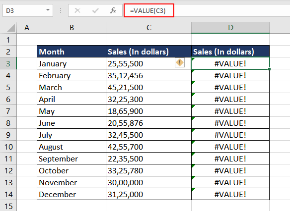
To be able to use the data for further calculations, we wish to convert them from text format to number format. As it is not an Excel-recognized format, the VALUE function will return a #VALUE! error.
To overcome this, we can first use the SUBSTITUTE function to replace all the commas with an empty string and then use the VALUE function. The formula used will be as follows.
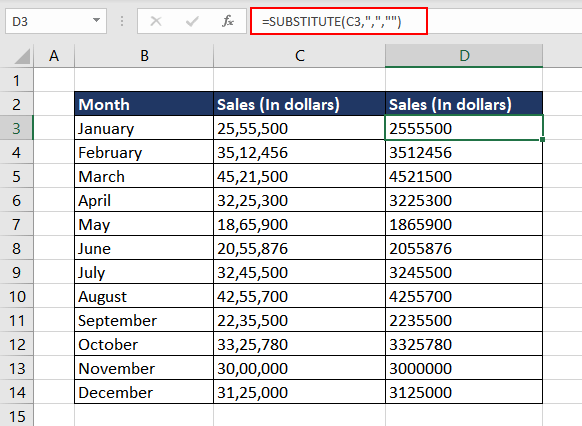
Now the sales values in column D are in a recognizable format i.e. text, with the help of the VALUE function, we can convert the same in number format. Combining both steps, the final formula used will be as follows.
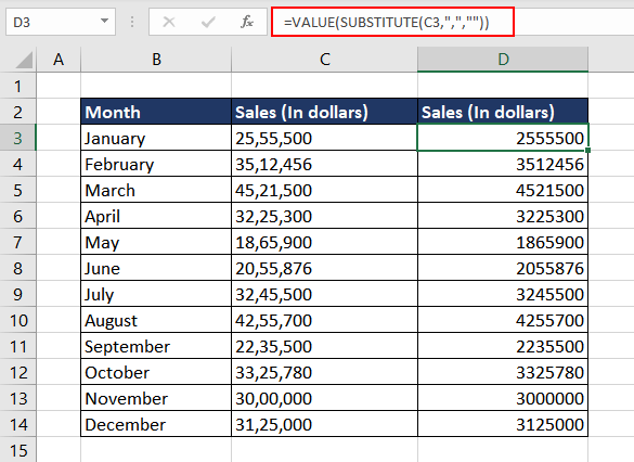
As evident by the right alignment of the data in column D, all the sales values are now in a number format and therefore can be further used for calculations.
Example 4 – Converting Time using the VALUE Function
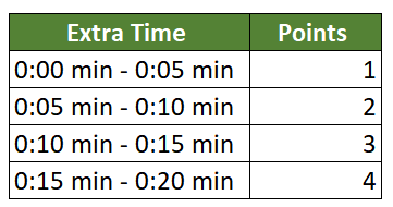
In this example, we are conducting an online test where the completion time is set to 10:00 AM. However, every applicant can take extra time up to 20 minutes, but points will be assigned depending on the extra time taken which will eventually be deducted from the actual score. Here are the points to be deducted as per the completion time.
As the first step, we will calculate the extra time taken in each case. The formula used will be as follows.
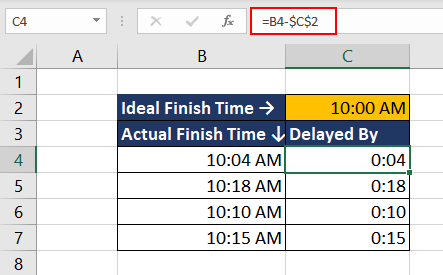
Now that we have all the values in column C, we can use the nested IF function to compare the time as per the point system and then assign the corresponding points. However, while using the delayed time data from C4:C7, we will wrap it in the VALUE function to ensure that Excel treats the time value as a number and not text.
The logic used will be as follows.
If the delayed time (C4) is less than 5 minutes, then assign 1 point, else if the delayed time is less than 10 minutes, assign 2 points….) and so on till 20 minutes. If no condition is met, the formula returns FALSE.
The formula used will be as follows.
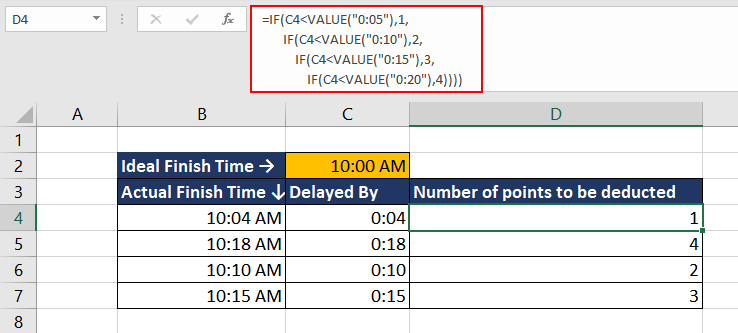
Now we have the final points that will be deducted from the final score in each case. With the help of the VALUE function, we were able to convert the time value from minutes to numerical format and execute the nested IF function.
VALUE Function vs NUMBERVALUE Function
Both the VALUE and NUMBERVALUE functions convert text that looks like a number from text format to numerical format but the NUMBERVALUE function transforms the data using the given group and decimal separators which help the function understand the format.
If the data is not in an Excel-recognized format, the VALUE function returns a #VALUE! error whereas with the NUMBERVALUE function, we can mention the group and decimal separator used in the data to convert it. Let's understand it better using an example.
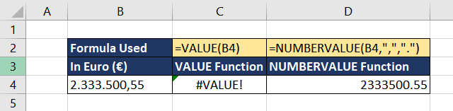
The data in cell B4 is a currency value in euros and is in a text format. The VALUE function does not recognize the data and hence throws a #VALUE! error whereas the NUMBERVALUE function converts the data from text to number format due to the mentioned decimal and group separator.
VALUE Function vs VALUETOTEXT Function
Now we know that the VALUE function converts text that looks like a number from the text format to numerical format. The VALUETOTEXT function performs the opposite conversion. The VALUETOTEXT function converts a value to text format depending on the concise or strict format.
Hopefully, now you have a clear idea about how to use the VALUE function to your advantage. Practice and discover new applications of the said function.
Subscribe and be a part of our 15,000+ member family!
Now subscribe to Excel Trick and get a free copy of our ebook «200+ Excel Shortcuts» (printable format) to catapult your productivity.
Value в excel что означает
Функция Excel VALUE помогает преобразовать текстовую строку, представляющую число (например, число, формат даты или времени) в число.

Синтаксис
=VALUE( text )
Аргумент
Текст (Обязательно): текст, который нужно преобразовать в число. Это может быть:
- Текст в кавычках;
- Или ссылку на ячейку, содержащую текст.
Возвращаемое значение
Функция Примечание
- #СТОИМОСТЬ! Ошибка возникает, если текст не является форматом числа, даты или времени, распознаваемым Microsoft Excel;
- Поскольку Excel автоматически преобразует текст в числовые значения по мере необходимости, обычно функция ЗНАЧЕНИЕ не требуется.
Пример
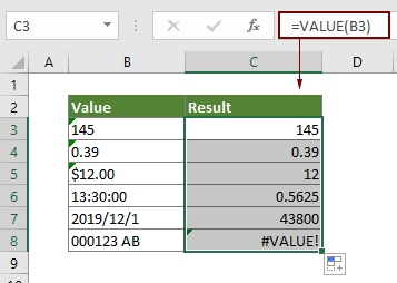
Как показано на скриншоте ниже, мы собираемся преобразовать список текстовой строки в числа. Функция VALUE может помочь в достижении этого.
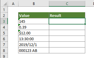
Выберите пустую ячейку, скопируйте в нее приведенную ниже формулу и затем перетащите маркер заполнения, чтобы применить формулу к другим ячейкам.
=VALUE(B3)
Связанные функции
Функция ПОДСТАВИТЬ в Excel
Функция ЗАМЕНА в Excel заменяет текст или символы в текстовой строке другим текстом или символами.
Функция Excel TEXT
Функция ТЕКСТ преобразует значение в текст с заданным форматом в Excel.
Функция Excel TEXTJOIN
Функция Excel TEXTJOIN объединяет несколько значений из строки, столбца или диапазона ячеек с определенным разделителем.
Функция Excel TRIM
Функция Excel TRIM удаляет все лишние пробелы из текстовой строки и сохраняет только отдельные пробелы между словами.
Функция ВЕРХНИЙ в Excel
Функция Excel ВЕРХНИЙ преобразует все буквы заданного текста в верхний регистр.
Лучшие инструменты для работы в офисе
Kutools for Excel — Помогает вам выделиться из толпы
Хотите быстро и качественно выполнять свою повседневную работу? Kutools for Excel предлагает 300 мощных расширенных функций (объединение книг, суммирование по цвету, разделение содержимого ячеек, преобразование даты и т. д.) и экономит для вас 80 % времени.
VALUE Function
The VALUE Function[1] is categorized under Excel Text functions. It will convert a text string that represents a number into a number. Thus, the function will convert text that appears in a recognized format (a number, date, or time format) into a numeric value.
In financial analysis, the VALUE function is not used much, as Excel automatically converts text to numeric values. However, it is important for anyone who wants to master the full extent of Excel functions.
Formula
=VALUE(Text)
- Text (required argument) – This is the text enclosed in quotation marks or a reference to a cell containing the text you want to convert.
How to use the VALUE Function in Excel?
The VALUE function was introduced in Excel 2007 and is available in all subsequent Excel versions. To understand the uses of the function, let us consider a few examples:
Example 1
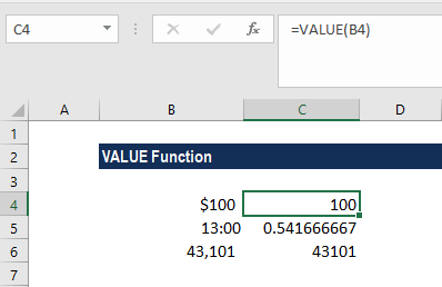
Let’s see how this function will behave when we give the following formulas:
We get the results below:
Example 2
Suppose an HR team wishes to assign a penalty point for an employee who arrives late. For assigning penalty points based on an amount of time tardy, you can use a nested IF formula.
Suppose we are given the data below:
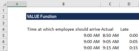
The formula to use is:
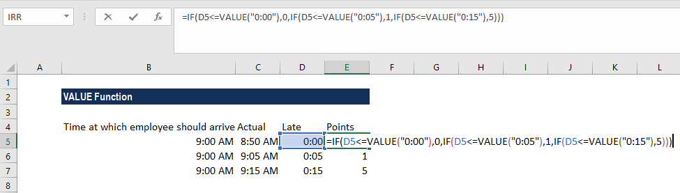
We get the results below:
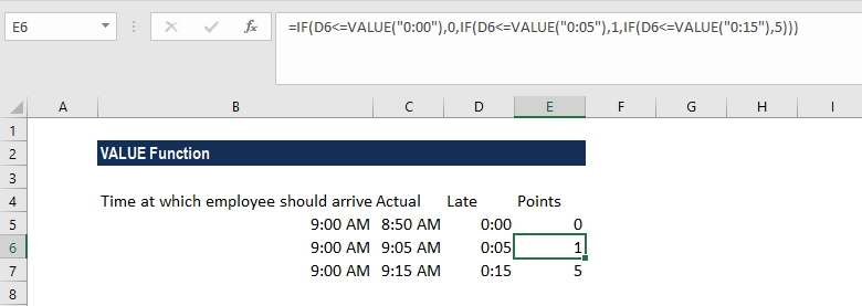
The formula first checks the tardiness by time in D5 to see if it’s 0, then zero points are assigned. If the result of the logical test above is FALSE, the formula checks to see if C3 is less than the next threshold, which is 5 minutes. It will then assign 1.
The same pattern repeats at each threshold. As the tests are run in order, from smallest to largest, there is no need for more complicated bracketing.
The VALUE function is used to make Excel treat the time value at each threshold as a number instead of next.
Things to remember about the VALUE Function
- As per Microsoft, the VALUE function is used for compatibility with other spreadsheet programs.
- The function converts text that appears in a recognized format (a number, date, or time format) into a numeric value.
Additional Resources
Thanks for reading CFI’s guide to this important Excel function. By taking the time to learn and master these functions, you’ll significantly speed up your financial analysis. To learn more, check out these additional CFI resources: